Past exam of the mathematics course of the University of Cambridge / 2003 / iii / Paper 42 / 3

Take logarithms entry by entry before centering. For tree $i$, let $z_i=(\log G_i,\log H_i,\log V_i{)}^T$, and put $\bar{z}=31^{-1}{\sum }_i{z}_i$. The command var(log(b)) computes the sample covariance matrix with the unbiased estimator normalizationThus entry $(j,k)$ is the sum of products of the centered log measurements divided by $30$, not the logarithm of the covariance between the original measurements. Its diagonal entries are the three log-variable sample variances, and the off-diagonal entries are their sample covariances. The positive off-diagonal entries indicate positive association of the log measurements. Taking logarithms turns a multiplicative relation such as $V\approx c{G}^{2}H$ into the approximately linear relation $\log V\approx \log c+2\log G+\log H$, which motivates investigating principal components of these transformed observations.

The command centres the log measurements and performs principal component analysis of their covariance matrix. With cor=F, it does not first standardize the variables to variance one. For a unit principal component loading vector $q$, the score $q^T(z_i-\bar{z})$ has sample variance $q^T\hat{\Sigma }q$. By the spectral theorem for real symmetric matrices, expand $q$ in an orthonormal eigenbasis; that variance is a weighted average of the eigenvalues. Its maximum is the largest eigenvalue, reached at the corresponding eigenvector. Repeating subject to orthogonality to previous directions gives the other principal components.

The software uses the divisor-$31$ sample covariance matrix for its component standard deviations, whereas var used divisor $30$. Diagonalizing the displayed matrix gives approximatelyTaking square roots of the latter gives $(0.5671603,0.07312405,0.03064834)$, agreeing with the output to the rounding of the displayed sample covariance matrix. The normalization changes these numerical standard deviations but leaves the eigenvectors and proportions of explained variance of a principal component unchanged.

The first principal component explains about $98.08\%$ of the total log-variable variance, the second another $1.63\%$, and the last about $0.286\%$. Keeping two preserves about $99.714\%$. An original scree plot displays the sharp drop after the first component:

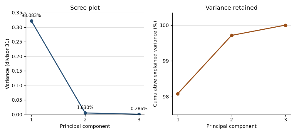
Consequently the centered cloud is very elongated along one direction: a one-dimensional approximation represents almost all of its squared variation. From the displayed covariance matrix, a unit first eigenvector, with its arbitrary sign chosen positive, is approximatelyIts principal component score is therefore $0.3980(\log G_i-\overline{\log G})+0.09514(\log H_i-\overline{\log H})+0.9124(\log V_i-\overline{\log V})$. All coefficients have the same sign, so this direction describes overall tree size, with log volume dominating the unstandardized variation. The summary alone supplies proportions, not the loading directions; the displayed sample covariance matrix supplies the latter. This is a geometric approximation, not evidence of an exact deterministic relation or independent original variables.

One further use is principal component analysis on a correlation matrix, obtained with cor=T, which equalizes marginal variances and answers a different scaling-sensitive question. Another is principal component regression: fit a response to selected principal component scores rather than highly correlated original predictors, choosing the number using prediction assessment. The fitted transformation also projects new measurements into the same low-dimensional coordinates, provided the training centering and scaling are retained.