Past exam of the mathematics course of the University of Cambridge / 2004 / iii / Paper 37 / 5

Use the time-homogeneous continuous-time multi-state model displayed in part ii. Write $Z(t)$ for the state at time $t$, $Q=(q_{rs})$ for its generator matrix, andFor $r\ne s$, $q_{rs}={\lim }_{h\downarrow 0}{p}_{rs}(h)/h$ is the transition intensity, and $q_{rr}=-{\sum }_{s\ne r}{q}_{rs}$. Condition on the observed initial state, and treat the clinic observation process and administrative end of follow-up as noninformative. A panel-observed interval contributes its transition probability, not the density of a jump at the examination date; the transitions inside that interval need not have been observed.

For the first patient, the two clinic intervals contribute $p_{11}(2)p_{13}(2)$. The subsequent death is observed at elapsed time $u=0.2$ after the last clinic state, so its contribution is the conditional death-time densityThe equality uses the permitted directions: starting from state 3, only living states 3 and 4 can be occupied before death. To obtain this density directly, survival in a living state $s$ until time $u$, followed by death in $(u,u+du)$, has probability $p_{3s}(u)q_{s5}du+o(du)$; add over the unobserved state $s$. Hence the mixed panel and exact-death likelihood contribution isIt includes the possibility of an unrecorded transition $3\to 4\to 5$ between the last clinic visit and death. Keeping only $p_{33}(0.2)q_{35}$ would exclude that allowed history, while $p_{35}(0.2)$ would be the probability of death by that time rather than the density of death at that time. With dates recorded in whole days, an exact interval-likelihood treatment integrates this density over the relevant day; the density formulation is its fine-time approximation.

For the second patient, the three successive intervals with state 1 at both ends, then the interval ending in state 2, and the last interval remaining in state 2 give the panel-observed multi-state likelihoodThere is no additional death contribution after the final administrative observation. Each likelihood contribution already accounts for being alive in the observed state at that visit. For independent patients their joint conditional likelihood contribution is $L_1{L}_2$.

For an explicit form, put ${\lambda }_r=-q_{rr}$. Irreversibility givesandThese formulas follow by integrating the density of the one possible intermediate jump time; at equal exit rates the limiting expression is $q_{rs}u{e}^{-{\lambda }_{r}u}$. ThusUsing the displayed fitted rates as numerical values gives $g_{35}(0.2)\approx 0.289314$ per year, $L_1\approx 0.017596$ per year and $L_2\approx 0.016048$, providing a check of the probability-versus-density distinction.

The permitted transitions form the following diagram. Each arrow is labelled by its fitted transition intensity in units of inverse years; the absence of an arrow is a structural restriction, not an estimated small effect.

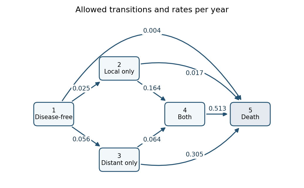
State 1 can move directly to 2, 3 or 5; state 2 can move to 4 or 5; state 3 can move to 4 or 5; and state 4 can move only to 5. There are no recovery transitions, and state 5 is an absorbing state. The rates of leaving the four living states are the sums of their outgoing arrows:The diagonal generator entries are their negatives, so every row of $Q$ sums to zero. These diagonal entries are not arrows or negative event rates. For example the direct $1\to 5$ rate is $0.004$ per year, while death after reaching another state can occur at a much larger rate. The printed fit has no covariates on the intensities, so it estimates one pooled rate system and contains no treatment-effect comparison, despite the trial's treatment randomization. The reported $-2\ell$ describes the fitted likelihood level; by itself it is not a goodness-of-fit test without a reference or competing model.

For a homogeneous continuous-time Markov chain, the holding time in a living state $r$ before the next transition has survival probability $e^{-{\lambda }_{r}t}$, where ${\lambda }_r={\sum }_{s\ne r}{q}_{rs}=-q_{rr}$. Indeed, conditional on still occupying that state, the probability of leaving in the next $dt$ is ${\lambda }_{r}dt+o(dt)$, so its survival function satisfies $S^{\prime }(t)=-{\lambda }_{r}S(t)$ and $S(0)=1$. Integrating gives the mean holding time from a transition intensity matrix:This is the mean time until any allowed exit from that state, not necessarily the patient's remaining lifetime.

For confidence limits, use the supplied standard error $s_r$ of the corresponding diagonal generator estimate. Changing its sign does not change its standard error, so it is also the standard error of ${\hat{\lambda }}_r$. The delta method, with derivative $d(1/\lambda )/d\lambda =-1/{\lambda }^2$, givesThe resulting approximate 95% Wald confidence intervals areThe diagonal standard errors already incorporate the covariance among outgoing rates. They should not be replaced by the square root of a sum of squared off-diagonal standard errors, which would silently assume those rate estimates independent.

Alternatively construct a positive rate confidence interval and apply the confidence interval for an inverse rate transformation. Here every normal rate interval has a positive lower endpoint, givingThese approximate intervals are, respectively, $(10.863,12.830)$, $(4.497,7.161)$, $(2.397,3.117)$ and $(1.548,2.631)$ years. They are asymmetric because inversion is nonlinear; positive log-rate or likelihood-based intervals could also be inverted. The symmetric delta intervals and the inverted-rate intervals are two legitimate first-order approaches and need not have numerically identical endpoints.

The death state has zero exit rate, so its holding time is infinite. There is no finite mean-sojourn estimate or ordinary finite confidence interval for this structurally absorbing state. All intervals above concern the mean parameter, not a prediction interval for one patient's realized holding time.

The transition matrix over five years is $P(5)=e^{5Q}$. Its first row conditions on starting in state 1. The displayed approximate probabilities mean that, five years later, about 65% remain disease-free, 6% have local recurrence only, 10% have distant metastasis only, 2% have both, and 16% have died. They are probabilities of the states occupied at five years; they are not the probabilities of the next jump destinations or annual transition intensities. In particular the positive probability of state 4 does not require a direct $1\to 4$ arrow: the paths $1\to 2\to 4$ and $1\to 3\to 4$ contribute to it. The probability of death includes deaths after any allowed sequence of intermediate states.

The printed row sums to $0.99$ rather than one because the entries are approximate; an exact stochastic transition row sums to one. Exponentiating the displayed three-decimal generator gives approximately $(0.65377,0.06490,0.09775,0.02532,0.15826)$, illustrating that the edited, low-precision table should not be treated as an exact matrix exponential of its separately rounded rates.

State 5 is an absorbing state, so once entered it can never be left. Its generator row is zero, and the last row of every positive-time transition matrix is thereforeThis explains all four leading zeroes in the printed last row.