Use signature and covariant one-particle state normalization . The future scattering condition uses the outgoing asymptotic scalar field:As with the incoming condition, this is understood in suitably smeared scattering matrix elements, not as unrestricted pointwise strong convergence of interacting and free local operators.
The free incoming field has expansionThe creation operator defines , with , so . On the other hand, translation invariance givesMatching the stable one-particle state component in the asymptotic condition fixes the constant overlap. Choose its state phase so that it is real and nonnegative. ThenThe same stable particle appears in the outgoing description, with compatible one-particle phases. Thus is the squared overlap measured by wave-function renormalization.
Insert a complete set of four-momentum eigenstates between the fields. For , translation invariance and Hermiticity giveFor , reversing the time-ordered product gives the same sum with . Therefore, with continuous-state integrals implicit in the completeness sum,Here is the Heaviside step function.
For the usual spectral representation, take a Lorentz-invariant vacuum, a positive-norm Hilbert space and the future-cone spectrum condition. Also take , as for the unbroken real scalar field, or subtract this constant and use the connected correlation function. Otherwise the vacuum intermediate state adds a disconnected constant not represented by the ordinary mass-shell measure below.
Let for that centered field, and use the Fourier transform convention . Define the Källén–Lehmann spectral density by the distributional equalityLorentz invariance makes the weight on each future mass shell a function or measure of ; the spectrum condition gives . Its nonnegativity follows from the displayed squared matrix elements. ThusApplying time ordering to this expression mass shell by mass shell proves the Källén–Lehmann spectral representation:The factor is outside under the convention in the question.
The stable one-particle state part of completeness is . Its overlap is , so its contribution to is times the free mass- two-point function. HenceOther isolated particles as well as multiparticle states can belong to . The full scalar propagator accordingly has isolated pole , making its pole residue.
Finally use canonical field normalization: the canonical momentum is and the equal-time canonical commutation relation is . The vacuum commutator has the same spectral decomposition. For each free mass shell,independently of . Comparing with the interacting equal-time commutator gives the canonical scalar spectral sum rule:For the particle genuinely interpolated by the stated asymptotic field, ; the general nonnegative bound allows a field with zero overlap. The total weight and the upper bound require this canonical normalization and a well-defined distributional equal-time limit. They do not follow from the asymptotic condition alone: rescaling rescales both and the entire spectral measure.
With signature , the momentum-space Feynman rules for phi-fourth theory follow by expanding the interaction exponential and using free-field Wick contractions. Every internal scalar propagator supplies , every quartic Feynman vertex supplies , and each vertex conserves four-momentum. Integrate every independent loop momentum with and divide by the Feynman-diagram symmetry factor . Equivalently, assign momenta to all lines and attach at each vertex before eliminating constrained integrations. A connected amputated graph therefore has the formwith the remaining overall momentum-conservation delta function understood. For an unamputated correlation function, retain the external propagators; scattering amplitudes instead use LSZ reduction. The factor in the interaction cancels the number of ways to attach the four identical fields at a vertex, leaving the stated vertex factor.
For a connected Feynman diagram, . The superficial degree of divergence is the power under simultaneous large rescaling of all independent loop momenta before considering cancellations or divergent subgraphs. Since each integration contributes four powers and each internal propagator removes two,Counting vertex half-edges gives . Substitution yieldsThe connectedness assumption matters: a disconnected interaction graph with components instead has the corresponding count . Tree graphs have no loop integral even when this formal power count is nonnegative.
In four dimensions the possible primitively divergent proper vertices have or , with or ; odd vertices vanish by the symmetry. The divergent local structures are a mass term, a kinetic term and a quartic coupling term. If vacuum diagrams are retained, a vacuum-energy term is also required. Thus one can renormalize using a finite family of operators already allowed by the theory's symmetries: four-dimensional phi-fourth theory is perturbatively renormalizable. The superficial count alone is not an all-orders convergence proof. After divergent subgraphs are subtracted with these counterterms, higher-point graphs have no new overall ultraviolet divergence; a negative overall does not by itself exclude subdivergences.
The requested lowest-order graphs and the three channels needed for the coupling correction are shown here:
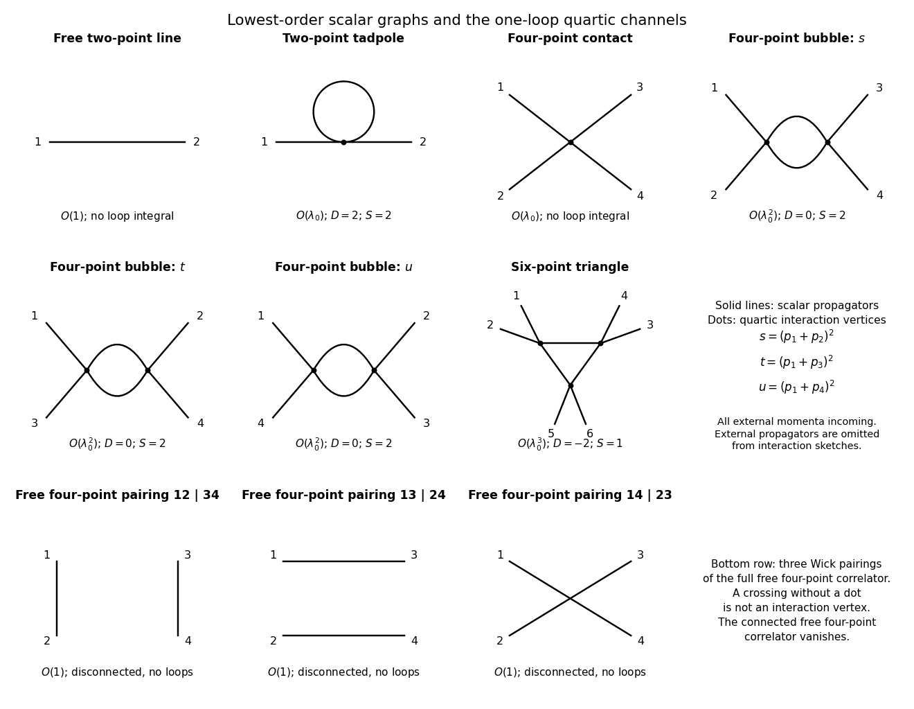
Original quartic-scalar diagrams: free line, tadpole, four-point contact and three bubble channels, ultraviolet-finite six-point triangle and all free four-point pairings
. Details. 
For the two-point function, the free propagator is order one, while its first interacting correction is the tadpole diagram, with , , and . Its loop integral behaves as and is quadratically divergent. For the connected four-point function, the lowest graph is the order- contact vertex, with and formal but no loop divergence. The first loop correction comprises the bubble diagrams. Each has , , and , matching its logarithmic integral .
If the full four-point correlation function rather than its connected part is considered, there is also an order-one contribution: the sum of the three Wick contractions into two free propagators, with pairings . Explicitly, , with the free scalar propagator between insertions . These disconnected pairings are drawn in the bottom row of the plate. They contain no loop integral and are not contributions to the proper four-point vertex.
A six-point amplitude in phi-fourth theory has a one-loop triangle Feynman diagram with two external legs at each of three vertices. It has , , and . For a fixed external-leg partition its loop integral contains three scalar denominators, for exampleAfter Wick rotation, its ultraviolet radial behavior is , which converges. The triangle has no proper loop subgraph, so no ultraviolet subdivergence is hidden in this example. It generates no new six-field counterterm. Nonzero mass avoids a separate infrared issue; with massless propagators exceptional external momenta can produce infrared singularities without changing this ultraviolet conclusion.
The bare mass is a coefficient in the regulated action, whereas the physical mass is the pole position of the full propagator. Write the amputated two-point insertion as . Summing its insertions givesAt order , only the tadpole contributes. Its factor one half follows directly from Wick pairing: of the four fields at the vertex, choices attach the two labeled external lines and the remaining pair closes the loop, so . ThusRotate through the Feynman contour. The from the measure and the in the propagator, together with the denominator sign, give a positive Euclidean integral. With spherical cutoff ,This is the Wick-rotated cutoff tadpole mass shift, and it is independent of external momentum. Hence to first order,For a positive stable quartic coupling the first-order shift is positive. Keeping the measured pole fixed while changing the cutoff requires adjusting the bare mass. At the bracket is understood by its finite limit . There is no momentum-dependent wave-function correction from this one-loop tadpole; such corrections begin at higher order.
Set and . The kinetic term gives the scalar mass dimension , so the quartic bare coupling has mass dimension . A dimensionless renormalized coupling therefore comes with the factor .
The order- proper four-point corrections are precisely the three bubble diagrams in the diagram plate, with external partitions . Each carries a symmetry factor one half. Its two-propagator integral has logarithmic ultraviolet divergence in four dimensions, represented in dimensional regularization by a simple pole at . That pole's residue is independent of external momenta, so a local quartic counterterm cancels it. The three channels add, rather than describing three separate couplings. The two-point tadpole has no momentum dependence, so it does not supply a one-loop field-normalization correction to the four-point coupling. The first momentum-dependent field correction contributes to this relation only at higher order.
With the supplied residue , the subtraction relation consequently readsA possible scheme-dependent finite subtraction does not change the displayed four-dimensional one-loop coefficient. Keep the regulator and bare coupling fixed while varying the renormalization scale, and define . Differentiation givesTo retain all quadratic terms, put . The engineering term times the pole factor contributes , and the remaining quadratic coefficient is . It vanishes only when . ThusDropping the product of the engineering term and pole factor would give the wrong sign for the loop term.
At , separation of the one-loop renormalization-group flow givesThereforeThis is the solution of the truncated one-loop equation, not an exact all-orders running law. It applies while the coupling remains sufficiently weak; its Landau pole is at for .
A renormalization-group fixed point has . For and a small perturbation , linearization givesThus means attraction as , or ultraviolet stability; means attraction as , or infrared stability. If the derivative vanishes, higher terms decide marginal stability. These statements concern the specified coupling direction; other couplings or the mass can be relevant even when this direction is stable.
For , the quadratic renormalization-group beta function has zeros and . At the nonzero zero,ConsequentlyThis is the weak-coupling Wilson-Fisher fixed point, perturbatively controlled near four dimensions. Reaching its full critical limit also requires tuning the mass, the thermal relevant direction at the Wilson-Fisher fixed point.
At , this nonzero fixed point merges with the Gaussian fixed point. Although the derivative at zero vanishes, for a positive weak coupling, so the running solution tends to zero logarithmically toward the infrared. The four-dimensional critical long-distance limit is Gaussian: the quartic interaction is marginally irrelevant, rather than flowing to a nonzero weakly interacting infrared fixed point. This is the Gaussian infrared limit of positive four-dimensional quartic coupling. It is not ultraviolet asymptotic freedom; the positive coupling grows in the ultraviolet. Nor does it say a massive theory has no interactions at finite energy: the critical or massless scaling regime is the one described by this limiting flow. Extrapolating the one-loop law to arbitrarily high cutoff at fixed positive low-energy coupling encounters its Landau pole; avoiding that pole as the cutoff is removed forces the perturbative coupling toward zero. This motivates the usual triviality conclusion, but the one-loop calculation alone is not a nonperturbative theorem excluding all possible strongly coupled ultraviolet completions.
For a constant unitary matrix , gives . Also , so the kinetic contraction is unchanged. The mass term and the squared norm in the potential are unchanged for the same reason. The original scalar action has the stated global symmetry. For a spacetime-dependent , however, , and the extra term prevents local invariance of the ordinary-derivative kinetic term.
Choose the gauge covariant derivative , with Hermitian. Demand . Expanding both sides yieldsso the necessary Yang-Mills gauge transformation isUnitarity makes the transformed connection Hermitian. This formula includes the inhomogeneous derivative term; mere conjugation would be insufficient for a local transformation.
Define the Yang-Mills field strength by . Direct expansion givesChoose an orthonormal Hermitian generator basis with . The compact simple Lie algebra has an invariant positive trace metric, so this basis can be chosen; its structure constants are totally antisymmetric. With these conventions a locally invariant dynamical action isEach matter contraction is invariant because transforms like , and the gauge kinetic term is invariant by cyclicity of the trace. It is in components. Choosing gives the familiar convention.
Formally introduce a gauge-field source and a normalized generating functionalA gauge-field Green function is obtained by source differentiation:Here is the unnormalized integral at zero source, so the normalized functional obeys . This expression needs gauge fixing: the integral repeats every physical configuration over its whole gauge orbit, producing an irrelevant but divergent gauge-group volume, and the free gauge kinetic operator has longitudinal zero modes, so it has no inverse propagator on that unrestricted space. Ordinary gauge-field Green functions are gauge-dependent; physical gauge-invariant quantities must be obtained consistently from the gauge-fixed theory.
Use the Lorenz condition . To keep signs explicit, parametrize a small transformation by , equivalently the original parameter is . The finite transformation above gives the adjoint gauge variation for a positive-sign covariant derivative:Therefore . Define the Faddeev-Popov operator as , absorbing the field-independent minus sign of its determinant into normalization.
In a perturbative gauge patch, with residual zero modes removed by boundary conditions, the Faddeev-Popov gauge-orbit identity isIt follows by changing coordinates from the gauge parameter to the gauge condition: the functional Jacobian is precisely the determinant of its linearization. Insert the identity into the integral and change variables along the orbit. The action and measure are invariant, so the gauge-group volume factors out and is divided away. Averaging the gauge-slice value with Gaussian weight changes the delta-functional restriction to the covariant gauge-fixing termThe remaining determinant depends on through . Omitting it while adding only would weight different orbits incorrectly.
For a finite matrix , expansion of a Grassmann integral selects the product containing every and . Anticommuting the variables into a fixed order attaches the sign of each permutation, giving proportional to , with only a matrix-independent phase. The regulated functional version therefore represents the Faddeev-Popov determinant asThe independent Faddeev-Popov ghost fields and antighost fields obey , with the corresponding mixed and antighost anticommutation. A commuting complex Gaussian integral instead gives an inverse determinant, so it cannot supply this Jacobian. The required local ghost term isAfter integration by parts,This exhibits the free ghost kinetic term and the ghost-gluon vertex. Ghosts are Grassmann-valued scalar auxiliary fields in the Adjoint representation, not physical fermionic particles or external asymptotic states. Their loop signs arise from anticommutation. In an Abelian theory the adjoint derivative loses the field-dependent part, so the determinant is field-independent and the ghosts decouple; in the non-Abelian theory they must be retained.
The correctly gauge-fixed source functional thus uses and integrates over . Expanding its interaction terms gives the gauge, matter and ghost vertices, and differentiating its source functional computes the gauge-field Green functions. For example, at non-null momentum the quadratic gauge kernel iswhere and are the transverse projector of a vector field and longitudinal projector of a vector field. With the Feynman prescription this gives the gauge-boson propagatorFor the chosen ghost normalization the quadratic kernel is , so the ghost propagator is . Redefining the antighost sign changes ghost propagator and vertex signs together, without changing the determinant or physical conclusions. Gauge fixing requires the accompanying determinant, and its local representation requires anticommuting ghost and antighost fields. The gauge-orbit argument is local/perturbative: global gauge copies, the Gribov ambiguity, prevent interpreting it as a globally unique gauge slice without further treatment.
Articles by others on the same topic
There are currently no matching articles.