Past exam of the mathematics course of the University of Cambridge / 2005 / iii / Paper 66 / 1

Write $B_j^n(t)=\left(\genfrac{}{}{0ex}{}{n}{j}\right)t^j(1-t{)}^{n-j}$ for the Bernstein basis, and set $B_j^n=0$ when $j$ is outside its index range. Differentiating and using $j\left(\genfrac{}{}{0ex}{}{n}{j}\right)=n\left(\genfrac{}{}{0ex}{}{n-1}{j-1}\right)$ and $(n-j)\left(\genfrac{}{}{0ex}{}{n}{j}\right)=n\left(\genfrac{}{}{0ex}{}{n-1}{j}\right)$ givesHence, after shifting the first sum by one index,Thus the derivative is a degree-at-most-$(n-1)$ Bézier curve whose control points are $n(P_{j+1}-P_j)$. They are vectors rather than necessarily positions on the original Bézier curve. This is the Bézier derivative control polygon.

Applying the preceding derivative identity repeatedly yields the Bézier derivative control polygon for every order:where the forward finite difference is $\Delta P_j=P_{j+1}-P_j$ andThe induction step multiplies by the remaining degree $n-r$ and takes one more finite difference. Derivatives above order $n$ vanish. In particular,If the actual parameter interval has length $h$ and $t$ is its normalized coordinate, derivatives in the original parameter acquire the additional factor $h^{-r}$. These formulas allow derivative evaluation and join tests using only the control polygon.

Let the first Bézier curve have degree $n$ and control points $P_0,\dots ,P_n$, and the next have degree $m$ and control points $Q_0,\dots ,Q_m$. Use one increasing parameter on the two adjacent intervals. For a continuous join, their endpoints must agree: $P_n=Q_0$. If each interval has length $h$, the endpoint derivatives are $n(P_n-P_{n-1})/h$ and $m(Q_1-Q_0)/h$. Therefore the parametric first-derivative join of Bézier curves is exactlyFor equal degrees, the two polygon edges incident on the common endpoint are equal vectors. Equivalently, $P_{n-1},P_n=Q_0,Q_1$ are collinear with the join as their midpoint. Agreement of edge directions without these lengths gives only geometric tangent continuity at a nonzero tangent, not equality of derivatives in the chosen parameter. The displayed condition also covers zero endpoint derivatives. With unequal interval lengths $h,k$, the condition is instead $n(P_n-P_{n-1})/h=m(Q_1-Q_0)/k$.

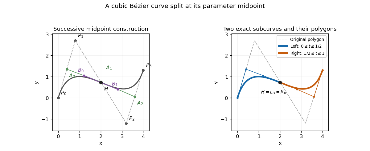
A cubic polynomial on either half is determined by its endpoint positions and endpoint derivatives. Use normalized parameters $s=2t$ on the first half and $s=2t-1$ on the second, so that derivatives with respect to $s$ are half the derivatives with respect to $t$. Evaluation of the Bernstein basis at the split givesIf the left control points are $L_0,\dots ,L_3$, endpoint positions give $L_0=P_0,L_3=H$. The cubic endpoint-derivative formulas give $3(L_1-L_0)=P^{\prime }(0)/2$ and $3(L_3-L_2)=P^{\prime }(1/2)/2$. On the right, $R_0=H,R_3=P_3$, $3(R_1-R_0)=P^{\prime }(1/2)/2$ and $3(R_3-R_2)=P^{\prime }(1)/2$. Substitution yieldsThese are exact restricted Bézier curves, since they match all four endpoint Hermite data of the respective cubics.

The construction is also the midpoint case of De Casteljau's algorithm. Form $A_j=(P_j+P_{j+1})/2$ for $j=0,1,2$, then $B_0=(A_0+A_1)/2$, $B_1=(A_1+A_2)/2$, and $H=(B_0+B_1)/2$. The two polygons are $(P_0,A_0,B_0,H)$ and $(H,B_1,A_2,P_3)$. Their common tangent edges satisfy $H-B_0=B_1-H$, as required for equal half-intervals. Thus the triangular midpoint construction simultaneously evaluates the split point and supplies the two exact representations.