Past exam of the mathematics course of the University of Cambridge / 2005 / iii / Paper 66 (Computer-aided Geometric Design)

Write $B_j^n(t)=\left(\genfrac{}{}{0ex}{}{n}{j}\right)t^j(1-t{)}^{n-j}$ for the Bernstein basis, and set $B_j^n=0$ when $j$ is outside its index range. Differentiating and using $j\left(\genfrac{}{}{0ex}{}{n}{j}\right)=n\left(\genfrac{}{}{0ex}{}{n-1}{j-1}\right)$ and $(n-j)\left(\genfrac{}{}{0ex}{}{n}{j}\right)=n\left(\genfrac{}{}{0ex}{}{n-1}{j}\right)$ givesHence, after shifting the first sum by one index,Thus the derivative is a degree-at-most-$(n-1)$ Bézier curve whose control points are $n(P_{j+1}-P_j)$. They are vectors rather than necessarily positions on the original Bézier curve. This is the Bézier derivative control polygon.

Applying the preceding derivative identity repeatedly yields the Bézier derivative control polygon for every order:where the forward finite difference is $\Delta P_j=P_{j+1}-P_j$ andThe induction step multiplies by the remaining degree $n-r$ and takes one more finite difference. Derivatives above order $n$ vanish. In particular,If the actual parameter interval has length $h$ and $t$ is its normalized coordinate, derivatives in the original parameter acquire the additional factor $h^{-r}$. These formulas allow derivative evaluation and join tests using only the control polygon.

Let the first Bézier curve have degree $n$ and control points $P_0,\dots ,P_n$, and the next have degree $m$ and control points $Q_0,\dots ,Q_m$. Use one increasing parameter on the two adjacent intervals. For a continuous join, their endpoints must agree: $P_n=Q_0$. If each interval has length $h$, the endpoint derivatives are $n(P_n-P_{n-1})/h$ and $m(Q_1-Q_0)/h$. Therefore the parametric first-derivative join of Bézier curves is exactlyFor equal degrees, the two polygon edges incident on the common endpoint are equal vectors. Equivalently, $P_{n-1},P_n=Q_0,Q_1$ are collinear with the join as their midpoint. Agreement of edge directions without these lengths gives only geometric tangent continuity at a nonzero tangent, not equality of derivatives in the chosen parameter. The displayed condition also covers zero endpoint derivatives. With unequal interval lengths $h,k$, the condition is instead $n(P_n-P_{n-1})/h=m(Q_1-Q_0)/k$.

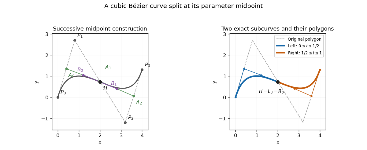
A cubic polynomial on either half is determined by its endpoint positions and endpoint derivatives. Use normalized parameters $s=2t$ on the first half and $s=2t-1$ on the second, so that derivatives with respect to $s$ are half the derivatives with respect to $t$. Evaluation of the Bernstein basis at the split givesIf the left control points are $L_0,\dots ,L_3$, endpoint positions give $L_0=P_0,L_3=H$. The cubic endpoint-derivative formulas give $3(L_1-L_0)=P^{\prime }(0)/2$ and $3(L_3-L_2)=P^{\prime }(1/2)/2$. On the right, $R_0=H,R_3=P_3$, $3(R_1-R_0)=P^{\prime }(1/2)/2$ and $3(R_3-R_2)=P^{\prime }(1)/2$. Substitution yieldsThese are exact restricted Bézier curves, since they match all four endpoint Hermite data of the respective cubics.

The construction is also the midpoint case of De Casteljau's algorithm. Form $A_j=(P_j+P_{j+1})/2$ for $j=0,1,2$, then $B_0=(A_0+A_1)/2$, $B_1=(A_1+A_2)/2$, and $H=(B_0+B_1)/2$. The two polygons are $(P_0,A_0,B_0,H)$ and $(H,B_1,A_2,P_3)$. Their common tangent edges satisfy $H-B_0=B_1-H$, as required for equal half-intervals. Thus the triangular midpoint construction simultaneously evaluates the split point and supplies the two exact representations.

Put $U=B_0-A_0$, $T=D_0-C_0$, $D=A_0-C_0$ and $v=V-W$. A point on each moving segment has the form $A_0+sU+tV$ and $C_0+rT+tW$, with $s,r\in [0,1]$. Contact is therefore equivalent toThe contact time of translating line segments is the minimum feasible $t$. This reduces the entire continuous-motion problem to three linear equations and linear inequalities.

In three-dimensional space form the matrix $H=[U,-T,v]$. If it is nonsingular, solveusing a stable linear solver. A candidate with $s,r$ in the unit interval and $t\ge 0$ is the only contact event and hence the earliest one; otherwise no contact occurs. Check initial intersection explicitly, so an already touching pair returns time zero.

If $H$ is singular, use a rank-revealing factorization to test consistency. Write every solution as $x=x_0+Nz$, with columns of $N$ spanning the null space, and minimize its time coordinate subject to the box and nonnegative-time constraints. This is a small linear programming problem. It handles parallel segments, collinear overlap, a continuum of contact times and segments degenerated to points. Infeasibility means no future contact. When $v=0$, the relative geometry is stationary: initially disjoint segments never meet. The first contact is the least feasible nonnegative time, not just an intersection of the two supporting lines.

The same relative coordinates give the proximity time of translating line segments asThis is a convex norm-constrained problem, rather than the linear feasibility problem for contact. One can solve it as a small second-order cone problem. If the distance between the initial line segments is at most $d$, the answer is zero; if no feasible point exists, the threshold is never reached.

For an elementary analytic algorithm, consider the nine combinations in which each of $s,r$ is either free, fixed at zero or fixed at one. In each case, minimize the squared distance over the free parameters. Writing $q(t)$ for $D+tv$ plus the fixed endpoint contributions, and $K$ for the columns belonging to free parameters, stationarity isIf the Gram matrix $K^{T}K$ is nonsingular, $z(t)=-(K^{T}K{)}^{-1}{K}^{T}q(t)$ is affine in time. Retain only the time interval on which its entries lie in $[0,1]$. The residual is then $r_0+t{r}_1$, and feasibility reduces toIntersect its solution interval with $t\ge 0$ and the free-parameter validity interval, and record the first point. Include the four endpoint–endpoint cases, where there are no unfixed segment parameters. Take the earliest valid candidate among all cases. The actual closest pair belongs to one of these faces of the parameter square, so this enumeration cannot miss the first approach.

The complications are the quadratic threshold equation, changes of the active closest-point feature and singular Gram matrices for parallel or degenerate segments. In a singular case, keep the affine family of minimizers and its feasibility bounds, or use the original convex problem; a pseudoinverse answer alone can fall outside the segment even when another minimizer is feasible. Constant-distance cases and tangential threshold contact must also be retained. Merely checking moving endpoints misses approaches between interior points.

Fix the indexing conventionwhere the subdivision arity $a>1$ is an integer. A change of the initial control $P_0^0$ can influence only indices $i=j_1$ after one step, where $M_{j_1}\ne 0$. After $\ell$ steps the possible descendant indices areLet $j_{\min },j_{\max }$ be the smallest and largest active subdivision mask indices. Dividing by $a^{\ell }$ gives the enclosureTherefore the support of a stationary subdivision scheme, in initial control-grid units, is enclosed byFor the stated symmetric subdivision mask with active extremes $-w,w$, the width is $2w/(a-1)$. For a nonzero compactly supported basic limit function $\varphi$, this is an exact endpoint calculation: its refinement equation is $\varphi (x)={\sum }_j{M}_j\varphi (ax-j)$. If $\beta$ is its right support endpoint, only the largest active subdivision mask index can contribute sufficiently close to the rightmost point of this sum; all smaller indices have argument beyond $\beta$. Hence $\beta =(\beta +j_{\max })/a$, giving $\beta =j_{\max }/(a-1)$. The left endpoint follows in the same way. This argument also excludes cancellation at an extreme for signed subdivision masks. The support for initial control $P_k$ is translated by $k$. If the nominal subdivision mask was padded by zero coefficients, use its actual extremes; and a limiting subdivision curve has to exist before its support is meaningful. This calculation describes the entire possible influence region, rather than the width of a single refinement stencil on its finer grid.

There are no numerical continuity bounds determined by $w$ and $a$ alone: the subdivision mask coefficients matter. First check constant reproduction, ${\sum }_j{M}_{ϵ-aj}=1$ for every residue $ϵ$, and convergence. For the usual stationary scalar scheme, two useful calculations are a uniform contraction test and a spectral obstruction test. Higher smoothness is tested with derived difference subdivision masks.

Write $M(z)={\sum }_j{M}_j{z}^j$ and $s_a(z)=1+z+\cdots +z^{a-1}$. Using backward differences $\Delta P_i=P_i-P_{i-1}$, the generating-function identityproves the subdivision difference scheme relation $\Delta S_M=S_{M/s_a}\Delta$. Iterating gives ${\Delta }^r{S}_M=S_{M/s_a^r}{\Delta }^r$. To test a candidate $C^r$ limit, suppose the requisite sum rules hold, so $M/s_a^{r+1}$ is a finite Laurent polynomial. The scaled derivative controls $q_i^{\ell }=a^{r\ell }{\Delta }^r{P}_i^{\ell }$ are refined by the subdivision maskwhose residue sums are one. Their first differences are refined byThe powers of $a$ are essential because each refinement shrinks parameter intervals by $a$.

A lower continuity bound comes from proving uniform contraction. The infinity norm of one difference-refinement step is bounded byIf $q<1$, adjacent derivative controls contract geometrically at every location. More generally, form the $p$-step subdivision maskand test ${\max }_{ϵ\mathrm{mod}{a}^p}{\sum }_j|(B_r^{[p]}{)}_{ϵ-a^{p}j}|<1$. This proves convergence of the constant-preserving derivative scheme to a continuous limit. One justification is to compare consecutive piecewise-linear interpolants: their difference is bounded by a constant times the maximum adjacent-control difference, and the geometrically decreasing bound is summable. To identify the limit as $P^{(r)}$, use fixed-degree Cardinal B-spline interpolants of the original refined controls. Their $r$th derivatives are sums of the scaled finite differences; convergence of both functions and derivatives gives $P\in C^r$. Testing successive $r$ supplies a guaranteed lower bound.

An upper continuity bound comes from an observable noncontracting shape mode. Build finite local subdivision matrices for $B_r$ on a refinement-invariant control neighborhood. For a digit $ϵ$ their entries are $(A_{ϵ}{)}_{ij}=(B_r{)}_{ϵ+i-aj}$, since the new index is $ak+ϵ+i$. Restrict to the realizable difference space and discard modes that do not affect the limit. A word ${ϵ}_1,\dots ,{ϵ}_p$ corresponds to a nested parameter location. If its product has an observable eigenvalue $\lambda$ with $|\lambda |>1$, repetition of this word makes some scaled derivative differences grow rather than tend to zero. For a stable limit representation, $C^r$ regularity would force these differences to vanish; hence general-position data cannot have $C^r$ continuity. A modulus-one mode requires examination of whether it actually persists, rather than an automatic rounding rule.

The two calculations can be organized through the joint spectral radius $\hat{\rho }$ of these restricted matrices:These norm and spectral bounds for subdivision regularity make the test computable from the subdivision mask. The right bound certifies all-word contraction when it is less than one; the left bound detects a repeated-word obstruction when it exceeds one. Longer products improve the tests. A single matrix's spectrum is not a substitute for controlling arbitrary products. The product estimates also appear in Charina's analysis of subdivision regularity; the strict contraction and observable-mode arguments above explain their respective roles.

A norm estimate controls the worst possible refined differences for every choice of the initial controls. Submultiplicativity turns a length-$p$ contraction into a bound for arbitrary long products, so it proves a certain number of continuous derivatives. Its absolute values can lose cancellations; failure of the estimate is inconclusive. It therefore gives a lower bound on smoothness.

Conversely, an observable eigenmode of a repeated local product exhibits a particular sequence of shrinking neighborhoods with inadequate decay. General-position controls have a nonzero coefficient in that mode, so greater derivative continuity is impossible. Special symmetric or polynomial data may suppress the bad mode; this is why the general-position qualification matters. The obstruction gives an upper bound on smoothness, while failure to find an obstruction proves nothing. A lower bound on spectral growth becomes an upper bound on smoothness because large surviving differences correspond to rough behavior.

For example, the binary Cardinal cubic B-spline subdivision mask has symbol $M(z)=(1+z{)}^4/8$, up to an irrelevant index shift. At derivative order $r=2$, the first-difference subdivision mask is $B_2=(1+z)/2$, whose maximum parity sum is $1/2$: the limit is at least $C^2$. At $r=3$, $B_3=1$, and the surviving difference mode does not decay. For generic controls the third derivative is piecewise constant with nonzero jumps, so the subdivision curve is not $C^3$. Here the lower and upper tests determine the exact integer continuity, but they need not coincide for an arbitrary subdivision mask. Stability, sum rules and borderline modes must be handled explicitly before interpreting any numerical estimate as a continuity level.

The tensor-product surface basis is $b_{jk}(u,v)={\varphi }_j(u){\psi }_k(v)$. If both univariate bases consist of nonnegative functions, thenIf both factors are strictly positive at the chosen parameters, their product is strictly positive there as well. Its support is the Cartesian product of the two factor supports. With partition of unity, this nonnegativity additionally places the parametric surface point in the convex hull of the active control points.

If each univariate basis sums to one, distribute the finite sums, or use local finiteness when the basis is infinite:Thus the tensor-product surface basis is a partition of unity. In particular, translating every control point by a fixed vector translates the parametric surface by precisely that vector, and constant control data produce a constant parametric surface.

Suppose ${\varphi }_j\in C^r$ in $u$ and ${\psi }_k\in C^s$ in $v$, including their respective knot joins. The mixed derivatives of the tensor-product surface basis areThese are continuous because each factor is continuous. A finite or locally finite control sum has the same property. In the usual total-order notation the parametric surface is therefore at least $C^{\min (r,s)}$, and also has the stronger stated rectangular set of continuous mixed derivatives. Across a $u$-knot its guaranteed order is $r$, and across a $v$-knot its guaranteed order is $s$. No general improvement over a factor's smoothness is possible: setting $P_{jk}=A_j$ and using ${\sum }_k{\psi }_k=1$ recovers the univariate curve ${\sum }_j{A}_j{\varphi }_j(u)$ as a parametric surface constant in $v$.

Let the univariate linear precision sites be ${\xi }_j,{\eta }_k$, meaningThen their Cartesian-product grid is a linear precision set for the tensor-product surface basis:Indeed, the first coordinate is $({\sum }_j{\xi }_j{\varphi }_j)({\sum }_k{\psi }_k)=u$, and the second is $({\sum }_j{\varphi }_j)({\sum }_k{\eta }_k{\psi }_k)=v$. More generally, take controls $P_{jk}=A+{\xi }_{j}B+{\eta }_{k}C$. The resulting parametric surface is exactlyThis proves linear precision of a geometric basis and affine map reproduction, including arbitrary changes of the embedding plane. In fact the products also reproduce the bilinear coordinate $uv$, since ${\sum }_{j,k}{\xi }_j{\eta }_k{\varphi }_j{\psi }_k=uv$; affine precision is the requested consequence.

The core parametric surface interrogation is evaluation of the position and its derivatives through second order:Position answers point queries; first derivatives give the differential, tangent directions and normal vector; second derivatives supply curvature. An evaluator should also report the parameter domain, patch adjacency, boundary curves and knot or crease locations, and whether these derivatives exist at the queried point. At a discontinuity boundary it should provide the relevant one-sided limits rather than silently average them.

For spatial searches, provide restriction or subdivision into equivalent smaller patches and certified bounding volumes, with error estimates when an approximate mesh is used. These allow intersection and closest-point algorithms to reject remote patches and refine the remaining candidates. A useful interface therefore combines differential evaluation with domain/topology and enclosure information. Inverse parameter lookup, ray intersection and nearest-point search can be built from these primitives using subdivision and local root or minimization solves; they need not be presumed exact basic evaluations of every representation.

Evaluate all quantities at $(u_0,v_0)$ and assume a regular surface point, $S_u\times S_v\ne 0$. The tangent plane passes through $S_0=S(u_0,v_0)$ and is spanned by $S_u,S_v$. ThusChoose the unit normal $n=(S_u\times S_v)/\Vert S_u\times S_v\Vert$. The first fundamental form has coefficientswhile the second fundamental form has coefficientsTo derive the curvature formula, differentiate $n\cdot S_u=n\cdot S_v=0$. This gives $-n_u\cdot S_u=e$, $-n_u\cdot S_v=f$, $-n_v\cdot S_u=f$ and $-n_v\cdot S_v=g$. Therefore the shape operator $-dn$, expressed in the tangent basis, isIts eigenvalues are the principal curvatures. Their product, the Gaussian curvature, is its determinant:Regularity ensures $EG-F^2=\Vert S_u\times S_v{\Vert }^2>0$. Reversing $n$ changes the signs of $e,f,g$ and both principal curvatures but leaves $K$ unchanged. At a singular parameter point this quotient and the cross-product normal vector are undefined; an alternative regular chart or separate geometric analysis is required.

A useful subdivision curve interrogation supplies the following connected capabilities. It describes the parameter interval, open or closed topology, endpoints and break points; it evaluates the limit point $C(t)$ and, where the scheme guarantees them, $C^{\prime }(t)$ and $C^{\prime \prime }(t)$; and it refines or restricts an interval while retaining the mapping to the original parameter. It also provides enclosing bounds and a certified curve-to-chord error on each restricted piece. These are enough to build clipping, intersections, closest-point searches, tangents, curvature and adaptive sampling.

The enquiries concern the subdivision limit, not just a finite refined control polygon. For a stationary local refinement matrix $A$, a limit vertex can be obtained from a normalized left eigenvector $w^{T}A=w^T$, $w^{T}1=1$, as $w^{T}P$. Derivatives use the appropriately scaled difference schemes or equivalent spline evaluation on regular intervals. The convergence and derivative hypotheses must actually hold for the scheme; no second derivative can be requested at an intrinsic crease.

If the subdivision mask is nonnegative and preserves constants, descendants and limit points lie in the relevant control-point convex hull, giving a useful enclosing volume. For subdivision masks with negative weights, that hull need not be an enclosure: the interface must supply another valid bound, for example from a proven refinement-error estimate. This distinction is important for safe spatial rejection in an algorithm.

The corresponding subdivision surface interrogation needs mesh connectivity and patch adjacency, boundary and crease flags, local coordinate charts with transition maps, and subdivision into smaller patches with their original-chart mappings. Its evaluation enquiry returns a limit point, tangent derivatives and a normal vector; second derivatives are supplied only where the limit is sufficiently smooth. Certified bounding volumes and patch approximation errors allow a hierarchy for intersection and proximity searches. Boundary-curve enquiries complete the interface for clipping.

On regular parts of a subdivision surface, these evaluations may use its equivalent tensor-product or box spline patch. Near an extraordinary subdivision vertex, the local subdivision matrix determines the limit position through its constant left eigenvector, and its tangent modes determine the normal vector under the scheme's characteristic map of a subdivision surface regularity conditions. Refinement alone does not establish those conditions. A subdivision surface may have a well-defined tangent plane there without possessing second derivatives or Gaussian curvature. An interrogation interface must distinguish these cases and can work on surrounding regular charts when a higher derivative is unavailable at the vertex itself.

Together, subdivision, bounds, topology and limit evaluation support ray–subdivision surface intersection: bounds eliminate irrelevant patches; surviving patches are refined, and regular candidate intersections are corrected using position and first derivatives. The returned intersection is a point of the limit subdivision surface with an error certificate, rather than automatically a point on the last control mesh.

Let the point light be at $L$. For a subdivision curve point $C(t)$, its projected shadow lies on the ray beyond the subdivision curve:The shadow is the first intersection of that ray with the receiving subdivision surface after the subdivision curve point. Thus solveand retain the smallest admissible $\lambda$. This is the defining equation for shadow tracing for a subdivision curve.

First organize the subdivision surface patches into a bounding volume hierarchy. For a restricted subdivision curve interval, rays through its enclosing volume define an enclosing ray cone from $L$; subdivision surface bounds that do not meet this cone can be rejected. Refine surviving subdivision curve intervals and subdivision surface patches. For a fixed $t$, isolate all possible ray intersections using those bounds, then correct each regular candidate with the Jacobian matrix for the Newton methodThe scalar triple product shows that $J$ is invertible exactly when $n\cdot (C(t)-L)\ne 0$. Enforce the patch domain and $\lambda >1$ throughout correction, and choose the smallest valid $\lambda$. Bounds or validated root isolation, rather than a fixed list of subdivision curve samples, are needed if every shadow component is to be found.

Once a regular intersection is known, follow it as $t$ changes. Differentiating $F=0$ gives a useful predictor:Take a small predictor step in $(u,v,\lambda )$ and apply a Newton method correction at the new subdivision curve parameter. Move through patch adjacency with its chart transition; shrink steps when derivatives or error estimates change rapidly. Subdivide further and test a geometric curve-to-chord bound to approximate the resulting shadow trace to a chosen tolerance.

Surface-boundary crossings terminate or clip a trace. If a ray has no admissible subdivision surface intersection, that subdivision curve parameter contributes no shadow on $S$. At grazing contact the Jacobian is singular, so use interval subdivision and root isolation to detect the event and seed any outgoing branches. If several intersections are possible, recheck which is first; facing the light locally is helpful but is not a proof of global uniqueness. Open-curve endpoints and closed-curve seams must also be accounted for. With a compact represented geometry, transversal intersections and validated subdivision bounds, this algorithm traces every visible component; a purely sampled implementation gives only a tolerance-dependent approximation and cannot certify arbitrary tiny missed components.

For a directional light, replace the ray by $C(t)+\lambda d$ for a fixed propagation vector $d$ and $\lambda >0$. The intersection equation becomes $S-C-\lambda d=0$, with Jacobian $[S_u,S_v,-d]$ and continuation right-hand side $C^{\prime }(t)$. The same enquiries and event handling apply.