Past exam of the mathematics course of the University of Cambridge / 2006 / iii / Paper 74 (Stellar and Planetary Magnetic Fields)

Write $D_t={\partial }_t+\mathbf{u}\cdot \nabla$ for the material derivative. The resistive induction equation, together with the solenoidal conditions on both fields, isSince $D_t\mathbf{x}=\mathbf{u}$, the product rule givesAlso $\Delta P=\mathbf{x}\cdot \Delta \mathbf{B}+2\nabla \cdot \mathbf{B}=\mathbf{x}\cdot \Delta \mathbf{B}$. Substitution proves the radial magnetic induction scalar equation:

In the insulating exterior the quasistatic magnetic field is current-free, so $\nabla \times \mathbf{B}=0$ and $\nabla \cdot \mathbf{B}=0$. Thus $\Delta \mathbf{B}=0$ and $\Delta P=0$ for $r>a$, with decay at infinity for an isolated field. This is an instantaneous exterior Laplace equation, rather than a diffusion equation with the interior value of $\eta$.

Use the usual nonmagnetic-interface assumptions: equal magnetic permeability on both sides and no surface current. The electromagnetic boundary conditions then make $B_r$ and the tangential magnetic field continuous. Hence $P=r{B}_r$ is continuous. In spherical coordinates, the solenoidal magnetic-field constraint readswhere the last term is the angular divergence on the unit sphere. Its right-hand side is also continuous, giving the insulating boundary condition for the radial magnetic scalar:Equivalently, the decaying exterior degree-$l$ spherical harmonic is proportional to $r^{-(l+1)}$, so its boundary amplitude satisfies ${\partial }_r{P}_{lm}(a)=-(l+1)P_{lm}(a)/a$.

Set $N={\int }_V{P}^{2}dV$, $D={\int }_{{\mathbb{R}}^3}|\nabla P{|}^{2}dV$, $M={\int }_{{\mathbb{R}}^3}|\mathbf{B}{|}^{2}dV$, and $q={\max }_V|Q|$. The confined flow satisfies the impermeability condition $\mathbf{u}\cdot \mathbf{n}=0$, so $Q=0$ at $r=a$. Multiplying the radial magnetic induction scalar equation by $P$ and integrating, the advection term vanishes by the divergence theorem:The same integration by parts, using $\nabla \cdot \mathbf{B}=0$, gives

For diffusion, Green's first identity in the sphere gives ${\int }_{V}P\Delta P=-{\int }_V|\nabla P{|}^2+{\int }_{\partial V}P{\partial }_{r}P$. In the exterior, $\Delta P=0$ and the normal on its inner boundary is $-\hat{\mathbf{r}}$, soThe infinity term vanishes for the isolated decaying field. The insulating boundary condition for the radial magnetic scalar permits matching the two traces, and therefore the exterior contribution is essential: it turns the diffusive term into $-\eta D$. Altogether,Applying the pointwise Cauchy-Schwarz inequality and then its integral version,Thus a nonzero field with stationary or growing $N$ must satisfy the radial-flow dynamo energy bound:

The temporal qualification matters. For general time-dependent dynamo action, nondecay does not make $N^{\prime }\ge 0$ at every instant; the boxed bound applies at nondecreasing instants, to a marginal or growing mode, or in an appropriate long-time sense. A uniform strict violation, $q\sqrt{M/D}\le \eta -\epsilon$ with $\epsilon >0$, gives $N^{\prime }\le -2\epsilon D$. The whole-space Sobolev inequality and Holder inequality give $N\le |V{|}^{2/3}\Vert P{\Vert }_6^2\le C_{a}D$, forcing exponential decay of $N$. Alternatively, for a bounded statistically steady field, time averaging the energy balance and applying Cauchy-Schwarz once more gives $q_{\ast }^2\ge {\eta }^2⟨D⟩/⟨M⟩$, where $q_{\ast }={\sup }_{t}q(t)$. Sustained dynamo action cannot have a uniform negative dissipation gap.

There is a minor operator misprint to resolve first. Interpreting $(\mathbf{x}\cdot \nabla {)}^2$ as composition, the Cartesian formula for the angular Laplacian isThe last term is missing from the printed Cartesian expression. For example, its truncated expression maps $x_1$ to $x_1$, whereas a degree-one spherical harmonic must have angular eigenvalue two. In what follows, use the stated angular spectrum $l(l+1)$ and the supplied poloidal-energy identity; these are consistent with the corrected operator.

The divergence theorem and the solenoidal magnetic-field constraint imply zero magnetic flux through every sphere. Consequently $P=r{B}_r$ has zero angular mean and no $l=0$ component. Expand in orthonormal spherical harmonics:By angular orthogonality, withthe gradient norm and the supplied poloidal-toroidal decomposition identity becomeSince $l(l+1)\ge 2$, this proves the poloidal magnetic energy bound by the radial scalar gradient:Equality holds when the radial scalar contains only degree-one angular components.

Define the poloidal and total magnetic energies by $E_P=M_P/(2{\mu }_0)$ and $E_{\mathrm{total}}=M/(2{\mu }_0)$. Combining the radial-flow dynamo energy bound with $D\ge 2M_P$ gives the necessary conditionIt has the same temporal interpretation as the bound in the preceding part; statistically steady versions use the corresponding time-averaged energies. It quantifies why dynamo action with a substantial poloidal fraction requires radial motion, while a purely tangential flow has $Q=0$.

Let $⟨\cdot ⟩$ denote the spatial average. Assume periodicity, or an equivalent homogeneous averaging limit in which total derivatives average to zero and integration by parts is valid. Fix the induced field to have zero mean. Expand the solution of the resistive induction equation in small magnetic Reynolds number:The uniform test magnetic field commutes with differentiation. Since $\Delta \mathbf{u}=-\mathbf{u}$, the first equation has solution ${\mathbf{b}}_1=(\mathbf{B}\cdot \nabla )\mathbf{u}$.

The quadratic second-order forcing need not be monochromatic, so one must not simply replace its inverse Laplacian by multiplication by $-1$. Instead use the self-adjointness of the Laplacian under the average:This proves the monochromatic small-Reynolds-number mean electromotive force expansion

For the symmetry of the first-order monochromatic alpha tensor, writeIts antisymmetric part is determined by contraction with the Levi-Civita symbol. The contraction identity givesThe second term vanishes by incompressibility; the first is $⟨{\partial }_j(u_j{u}_p)⟩=0$. Since every three-dimensional antisymmetric second-rank tensor is equivalent to its contracted axial vector, ${\alpha }^{(1)}$ is symmetric. No Fourier series or Fourier transform is required.

To derive the next identity, set $\mathbf{C}=\mathbf{u}\times (\mathbf{B}\cdot \nabla )\mathbf{u}$. Expanding the curl and cross product in components,The average of the second term is zero: integration by parts makes it $-⟨C_i{\partial }_j{u}_j⟩$. Integrating the first term by parts givesExtracting the coefficient of $B_j$ now yieldsInterchanging $i$ and $j$ reverses the cross product, proving the antisymmetry of the second-order monochromatic alpha tensor:The second coefficient of the alpha tensor can therefore contribute turbulent magnetic pumping, while its symmetric part vanishes at this order.

Let ${\rho }_0$ be the reference mass density, $\nu$ the kinematic viscosity, $\kappa$ the thermal diffusivity, $\eta$ the magnetic diffusivity, and ${\alpha }_T$ the coefficient of thermal expansion. The conductive state of Rayleigh-Bénard convection is $T_b=T_0+\Delta T(1-z/d)$. For the Boussinesq approximation, density variation is retained only in buoyancy. Linearizing about this state and the imposed magnetic field $B_0\hat{\mathbf{y}}$ givesHere $w=u_z$ and $p_{\ast }=p^{\prime }+B_0{b}_y/{\mu }_0$ is the perturbation of magnetohydrodynamic total pressure. The gradient part of the Lorentz force has been absorbed into $p_{\ast }$; the remaining term is magnetic tension. The sign in the temperature equation follows from $d{T}_b/dz=-\Delta T/d$.

Use the thermal-diffusion scaling of a convection layer: length $d$, time $d^2/\kappa$, velocity $\kappa /d$, temperature perturbation $\Delta T$, field perturbation $B_0$, and total-pressure perturbation ${\rho }_0\nu \kappa /d^2$. Dropping dimensionless-variable decorations giveswithThese are respectively the Rayleigh number, Chandrasekhar number, Prandtl number, and magnetic-to-thermal diffusivity ratio. In particular, the magnetic coefficient is $\zeta Q$, not $Q$ alone, in these thermal-time units. At $z=0,1$, the boundary conditions are $\theta =w=b_z=0$, ${\partial }_z{u}_x={\partial }_z{u}_y=0$, and ${\partial }_z{b}_x={\partial }_z{b}_y=0$.

Put $a_h^2=k^2+m^2>0$ and $\Lambda =a_h^2+{\pi }^2$. The plane-layer poloidal-toroidal decomposition supplies the assumed poloidal fields asSince $w=-{\Delta }_h\varphi$ and $b_z=-{\Delta }_h\chi$, potentials proportional to $e^{st+ikx+imy}\sin \pi z$ have the required vertical components. Their horizontal components are proportional to $\cos \pi z$, satisfying the stress-free boundary conditions and the horizontal-field boundary conditions. The double-curl representation automatically enforces incompressibility and the solenoidal magnetic-field constraint.

Let $W,\Theta ,C$ be the amplitudes of $w,\theta ,b_z$. The temperature and resistive induction equations immediately giveEliminate the total-pressure perturbation by applying $\Delta$ to the vertical momentum equation and subtracting ${\partial }_z$ times its divergence. The resulting vertical equation isIn particular, $imC=-m^{2}W/(s+\zeta \Lambda )$ shows explicitly that magnetic tension opposes the displacement.

Taking the determinant of these three amplitude equations gives the horizontal-field magnetoconvection dispersion relation:This cubic polynomial includes all roots of the assumed poloidal coupled system; using its determinant form avoids discarding possible roots by dividing by $s+\Lambda$ or $s+\zeta \Lambda$. As a check, $Q{m}^2=0$ factors off magnetic diffusion and leaves the standard stress-free Rayleigh-Bénard convection growth equation.

Set $s=0$ in the horizontal-field magnetoconvection dispersion relation. With positive $\sigma ,\zeta$ and nonzero $a_h$, cancellation gives the stationary neutral curveAt fixed $a_h^2$, the Chandrasekhar number contributes a nonnegative penalty proportional to $m^2$. It can be eliminated by choosing $m=0$. It remains to minimize $f(x)=(x+{\pi }^2{)}^3/x$ for $x=k^2>0$:The function diverges at both endpoints and has its unique minimum at $x={\pi }^2/2$. Thus the magnetic-field-aligned rolls evade steady magnetic inhibition:independently of $Q$. If higher vertical sine modes are included, replacing $\pi$ by $n\pi$ gives minimum $27n^4{\pi }^4/4$, so the displayed first vertical mode also gives the smallest steady threshold.

Physically, these convection rolls have axes along the imposed magnetic field. Their perturbations are independent of $y$, so ${\partial }_y\mathbf{u}=0$ in the resistive induction equation and no growing magnetic perturbation is generated. The flow does not bend the field; consequently magnetic tension cannot inhibit these rolls, however large the field strength. This conclusion concerns the requested steady disturbances.

For disturbances varying only along the imposed magnetic field, set $k=0$ and $x=m^2>0$. The steady horizontal-field magnetoconvection dispersion relation becomesExpand it in powers of $x$:Its derivative and second derivative areBecause $R$ diverges as $x\to 0$ and $x\to \infty$, the unique minimum is determined byFor large Chandrasekhar number, this equation first gives $x\sim {\pi }^3{Q}^{-1/2}$ and hence the requested strong-field steady magnetoconvection varying along the field selection law:

For the threshold through order unity, the leading $Qx+{\pi }^6/x$ contribution at its optimum is $2{\pi }^3\sqrt{Q}$. More precisely, the stationary equation givesThe correction to $Qx+{\pi }^6/x$ has no first-order contribution because that expression is already stationary at its leading minimizer. Also $3{\pi }^{2}x=O(Q^{-1/2})$ and $x^2=O(Q^{-1})$. ThereforeThe constant term $3{\pi }^4$ must be retained. This restricted family bends magnetic field lines, so its large stationary threshold is compatible with the unrestricted field-aligned minimum in the preceding part.

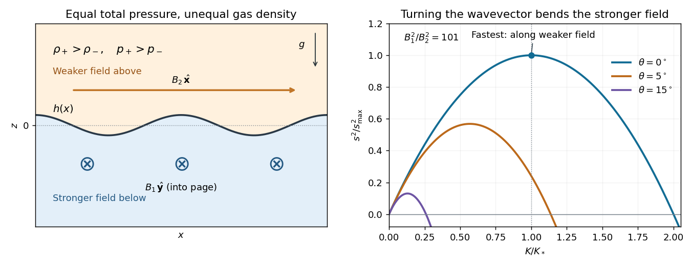
Write $c_T^2=\mathcal{R}{T}_0$ for the squared isothermal sound speed, distinguishing the gas constant $\mathcal{R}$ from a Rayleigh number, and put $H=c_T^2/g$. A uniform magnetic field has no bulk Lorentz force, so hydrostatic equilibrium and the ideal gas equation giveAt the interface, it is magnetohydrodynamic total pressure, not gas pressure alone, that is continuous:Define ${\Delta }_B=B_1^2-B_2^2>0$. The magnetic pressure discontinuity in an isothermal atmosphere therefore producesIn particular, the upper gas is denser at the interface. Both halves have the same scale height $H$, despite their different pressure normalizations.

For the disturbance calculation, write ${\rho }_{-}=\rho$, ${\rho }_{+}=\rho +\delta \rho$, where $\delta \rho ={\Delta }_B/(2{\mu }_0{c}_T^2)$, and ${\Sigma }_{\rho }={\rho }_{-}+{\rho }_{+}$. Work to leading order in the prescribed short-vertical-scale approximation: the bulk motion is locally incompressible potential flow, while the isothermal equation determines the equilibrium density jump. Its scale separation and small compressive correction will be checked at the maximizing mode.

Let the interface displacement be $h{e}^{st+ikx+imy}$ and $K=\sqrt{k^2+m^2}>0$. Using displacement rather than velocity potentials, write ${\mathbf{\xi }}_i=\nabla {\chi }_i$ and ${\mathbf{u}}_i=s{\mathbf{\xi }}_i$. Incompressibility and irrotational flow give $\Delta {\chi }_i=0$. Decay away from the interface and continuity of its normal displacement fixwith the common horizontal and temporal exponential understood. Both satisfy ${\partial }_z{\chi }_i(0)=h$. Thus the disturbance has vertical extent of order $K^{-1}$.

In ideal magnetohydrodynamics, magnetic flux freezing gives ${\mathbf{b}}_i=({\mathbf{B}}_i\cdot \nabla ){\mathbf{\xi }}_i$ for these locally incompressible displacements. If ${\pi }_i=p_i^{\prime }+{\mathbf{B}}_i\cdot {\mathbf{b}}_i/{\mu }_0$ is the total-pressure perturbation, linear momentum isSince $({\mathbf{B}}_i\cdot \nabla {)}^2=-({\mathbf{k}}_h\cdot {\mathbf{B}}_i{)}^2$ on the mode, integration in each half-space yieldsAt the displaced interface, continuity of Lagrangian magnetohydrodynamic total pressure requires ${\pi }_1-{\rho }_{-}gh={\pi }_2-{\rho }_{+}gh$. Inserting the two potentials gives the orthogonal-field magnetic Rayleigh-Taylor dispersion relation:The first term is the destabilizing Rayleigh-Taylor instability of the heavier upper gas; the second is stabilizing magnetic tension. A negative right-hand side gives an oscillatory mode rather than growth.

For fixed $K$, the magnetic penalty isIt is minimized by $m=0$: the wavevector is along the weaker upper magnetic field and perpendicular to the stronger lower field. If $B_2\ne 0$, define $A=g\delta \rho /{\Sigma }_{\rho }$ and $C=B_2^2/({\mu }_0{\Sigma }_{\rho })$. The growth law for this orientation is $s^2=AK-C{K}^2$, a concave quadratic with maximum at $K_{\ast }=A/(2C)$. HenceFor this orientation the unstable interval is $0<K<2K_{\ast }$; the maximum lies halfway along it.

The localization condition for the fastest orthogonal-field interface mode follows directly from the vertical decay length:This is the condition for ${\ell }_{\ast }\ll H$ on both sides. It also controls the locally incompressible approximation, sinceAcoustic adjustment is then fast compared with growth, so bulk density perturbations are higher-order corrections. If this localization condition fails, the constant-background approximation cannot be used to identify the physical fastest mode.

Finally, the printed assumptions allow $B_2=0$. In that case $m=0$ eliminates magnetic tension on both sides and gives $s^2=g\delta \rho |k|/{\Sigma }_{\rho }$. There is no finite maximum growth rate or maximizing wavenumber in the ideal sharp-interface model: growth is unbounded as $|k|\to \infty$. The finite maximum and localization formula above therefore require $0<|B_2|<|B_1|$.

In the growth curves, $\theta$ is the angle of the horizontal wavevector from the $x$-axis. The illustrated ratio $B_1^2/B_2^2=101$ gives $K_{\ast }H=25$, and shows how even a small rotation toward the stronger magnetic field lowers the maximum growth.