In this static scalar problem, a classical field-theory soliton is a nontrivial smooth localized finite-energy field configuration which is static in its rest frame and stable against admissible small perturbations. Moving examples are obtained by a Lorentz boost. The relevant static energy isUse the usual vacuum normalization , with zero energy at a vacuum, and impose finite-energy vacuum behavior at spatial infinity. These assumptions, together with the unconstrained real target and the canonical two-derivative kinetic term, are the hypotheses of the following Derrick theorem argument.
For Derrick scaling , change variables to obtainA static solution must be stationary under this admissible scale variation. The Derrick virial identity isFor , both terms are nonpositive and the gradient term is strictly negative for a nonconstant field, so no nontrivial static solution is possible. At , the identity forces , but the gradient term is scale invariant and a further argument is needed.
Since , implies everywhere. Every zero of a differentiable nonnegative potential has . The static Euler-Lagrange field equation therefore makes a harmonic function. Each derivative is harmonic and belongs to L2 space by finite energy. Its mean-value property and the Cauchy-Schwarz inequality on a ball of radius implyLetting gives . This proves the two-dimensional flat-target Derrick obstruction. Thus a nontrivial static real-scalar soliton in this class can occur only for . The argument does not apply unchanged to curved-target sigma models or gauge-field energies.
In one dimension the scale identity is , and the second scale derivative is for a nontrivial solution; scale variation does not rule it out. To derive the Bogomolny equations, write on the field interval of interest. Completing the square givesTherefore the Bogomolny bound and its saturation equation areEquivalently, for a monotone field connecting adjacent vacua, , with the sign chosen for its direction. Differentiating the first-order equation gives , verifying the static Euler-Lagrange field equation. Saturation minimizes energy within the fixed-boundary topological sector.
For the given sextic potential, factorization gives , so the vacua are . ChooseThis choice satisfies . On , the increasing kink in a phi-six model satisfies . Setting gives . Separation givesand henceThe endpoints are zero and two, and the mass follows from . The other increasing elementary scalar-field kink isIt uses the opposite sign of and has the same mass. Reflecting yields the two decreasing antikinks; is the free center.
There is no single finite-width static kink directly connecting to . Multiplying the static equation by gives the first integral for a finite-energy vacuum-to-vacuum solution. At the intermediate vacuum , this forces . Uniqueness for the smooth second-order field equation makes data stay at that vacuum, so a nontrivial solution cannot cross it at finite . This is the intermediate-vacuum obstruction to a kink; the two elementary transitions can only separate by an infinite interval.
A nonlinear sigma model describes a field taking values in a Riemannian target rather than an unconstrained linear space. Its static configurations are harmonic maps, critical points of the Dirichlet energy. The standard example for sigma-model lumps is the O3 nonlinear sigma model in two spatial dimensions: a unit vector hasThe same target is the complex projective line, giving the CP1 nonlinear sigma model description. A lump is a localized finite-energy static solution, whose existence and minimum energy are governed by the degree of its field map.
Impose a fixed angle-independent value at spatial infinity and require the field to extend smoothly there. The one-point compactification of the plane is a sphere, so the configuration becomes a map . Its topological degree is the integerThis is the degree charge of an O3 sigma-model lump: the integrand is the pullback of the oriented unit-sphere area form, normalized by its area . Equivalently, the degree counts inverse images of a regular target point with orientation signs. It is unchanged under smooth homotopy with the prescribed boundary value. Consequently fields of different degree belong to distinct topological sectors.
Topology also determines an energy lower bound. The derivatives are tangent to the sphere, so . Since
, square completion givesChoosing the sign of proves the Bogomolny degree bound for the O3 sigma modelFor positive degree, equality holds precisely when ; for negative degree the opposite sign applies. These are the Bogomolny equations for the lump. A saturating field minimizes energy in its degree sector and hence solves the static field equation. Explicitly, that equation is , obtained by varying under .
, square completion givesChoosing the sign of proves the Bogomolny degree bound for the O3 sigma modelFor positive degree, equality holds precisely when ; for negative degree the opposite sign applies. These are the Bogomolny equations for the lump. A saturating field minimizes energy in its degree sector and hence solves the static field equation. Explicitly, that equation is , obtained by varying under .
The first-order equations become especially simple in stereographic projection. Use andThe round target metric is . In the one-half energy normalization used here, the stereographic energy of the O3 sigma model and degree areThus . Positive-degree lumps are holomorphic maps, , and negative-degree lumps are antiholomorphic maps, .
A holomorphic sphere map is meromorphic in a stereographic coordinate and hence a rational map with coprime polynomials. To see why the rational form suffices, its finitely many coordinate poles can be removed by subtracting their principal parts, leaving a holomorphic function on the compact sphere and therefore a constant. The degree of a rational map of the Riemann sphere isafter canceling common factors. A generic target value has inverse images solving , with the root at infinity counted in homogeneous coordinates when necessary; the number is , and holomorphic local degrees are positive. Poles of do not make the physical field singular: the reciprocal target coordinate is regular there. Antiholomorphic rational maps have the opposite topological degree and the same minimum energy.
For example, the unit sigma-model lump and size modulus isIts degree is one and radial integration gives . The complex center supplies two position parameters, while the magnitude and phase of give size and internal orientation. More generally, fixing allows a monic degree- denominator and a numerator of degree at most , with no common roots. Their complex coefficients give the based rational-map moduli of sigma-model lumps.
Two-dimensional Derrick scaling leaves this pure-gradient energy unchanged, so degree fixes the minimum energy but not a preferred size. As , the unit-lump energy concentrates and the field limit is singular at its center. A degree cannot change through a smooth boundary-preserving deformation, but concentration can leave that smooth configuration space. Thus topological degree protects the smooth sector and determines the Bogomolny energy, while not by itself stabilizing the lump size. There is no contradiction with the scalar obstruction in Question 1: a curved-target harmonic map obeys a nonlinear constrained field equation, rather than having harmonic unconstrained components.
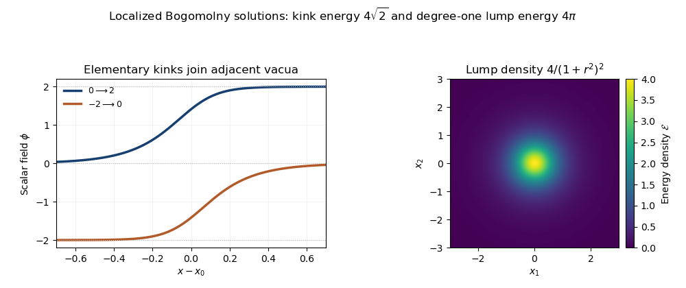
Adjacent-vacuum phi-six kink profiles and the localized energy density of a degree-one sigma-model lump
. Details. 
The kink panel uses the normalization of Question 1. The lump panel has and in the unit sigma-model lump and size modulus; changing its size redistributes the density while keeping its total energy .
Use anti-Hermitian matrices, with invariant positive inner product . On an adjoint-valued field , define the adjoint covariant derivative and gauge curvature byEquivalently, and . Put , with . The monopole Bogomolny equations are .
For a smooth SU(2) gauge transformation , useDifferentiating a transformed adjoint field shows : the derivatives of cancel the inhomogeneous term in . Applying the commutator of these derivatives gives , and therefore . Both sides of transform identically, establishing gauge invariance of the solution condition. Individual matrix components are covariant, rather than invariant numbers.
The monopole boundary condition is a nonzero asymptotic Higgs norm,together with finite three-dimensional Yang-Mills-Higgs energy. Standard monopole asymptotics have and . The normalized Higgs field at infinity defines a map , whose topological degree is the magnetic charge. A nonzero charge gives a genuine non-Abelian magnetic monopole; the nonzero Higgs boundary value alone also allows the zero-charge vacuum. Thus the relevant nontrivial solutions are Bogomolny-Prasad-Sommerfield monopoles in the zero-Higgs-potential limit.
Now form the four-dimensional connection with -independent components. Its gauge curvature hasThe self-duality sign requires an orientation. Choose the Euclidean metric and orientation . For cyclic , the Hodge star operator satisfiesUsing and , the curvature isEach term has negative star eigenvalue, soThis proves the Anti-self-dual Yang-Mills equations in the stated convention. The orientation of a monopole lift matters: with instead, the same connection is self-dual. With that opposite orientation, the anti-self-dual lift would use .
To fix the action normalization, take the Euclidean Yang-Mills actionBoth sums are over ordered index pairs. The component identity
givesHence the four-dimensional action density in terms of the three-dimensional curvature isA different overall action normalization rescales all three equal expressions together.
givesHence the four-dimensional action density in terms of the three-dimensional curvature isA different overall action normalization rescales all three equal expressions together.
A Yang-Mills instanton is a smooth finite-Euclidean-action self-dual or anti-self-dual connection in pure Yang-Mills theory, with the usual asymptotic pure-gauge behavior. Physically the term generally refers to a nontrivial field; its asymptotic gauge winding labels an instanton number. The Bianchi identity , together with , implies , so the first-order equations already imply the second-order Yang-Mills equations. Finite action is a separate requirement.
Here is independent of . If the monopole has nonzero curvature, the density is positive on an open set in , and integrating its infinite -extent givesFor a finite-energy monopole this can also be written as its positive action per unit length times . Thus a nontrivial monopole lift is not a Yang-Mills instanton on . The flat solution , constant is the zero-action exception: it is a vacuum, or a trivial charge-zero instanton if that terminology includes flat connections. It is not a counterexample to the nontrivial-monopole assertion.
More generally, finite Yang-Mills action forbids nontrivial translation symmetry, even when the translation preserves a connection only up to gauge. Such a symmetry would preserve its positive gauge-invariant action density. A nonflat field has a ball on which this density is bounded below by some positive constant. Repeated translations by a nonzero symmetry vector produce infinitely many disjoint copies of a sufficiently small such ball, all with the same positive action contribution, contradicting finiteness. Continuous translation invariance is a special case. Therefore a nonflat ASDYM instanton is localized in all four Euclidean directions and has no nonzero translational symmetry. Translating an instanton still produces another instanton with a shifted center; these position parameters belong to the instanton moduli space, rather than being invariances of one localized solution.
Let be homogeneous coordinates on the complex projective line. The complex tautological line bundle has fibre the line over that point. Its dual is the hyperplane line bundle . Define the tensor powers of the hyperplane line bundle by for , the trivial line bundle for , and the appropriate power of for .
An explicit holomorphic line bundle construction uses the two charts and with coordinates and . Choose holomorphic local frames related on the overlap byThis is consistent with the tautological frames and for . A holomorphic section of is represented by entire chart functions satisfyingExpand . Holomorphicity of at requires every power with to vanish. Thus for , is exactly a polynomial of degree at most . Conversely every such polynomial gives an entire . Its coefficients supply the explicit isomorphismEquivalently, the global holomorphic sections are the homogeneous polynomials . For , the same chart argument gives no nonzero global section.
For the first cohomology, use the sheaf of holomorphic sections of a vector bundle and its Čech cohomology on this two-chart cover. A zero-cochain is a pair of entire chart functions . A one-cochain is a function holomorphic on , multiplied by . There are no alternating two-cochains on a two-set cover, so every one-cochain is a cocycle. The coboundaries areConsequently the holomorphic Laurent-series cohomology of twists on the projective line isHere the last term means the set of functions with entire. The charts and their intersection are Stein manifolds; Cartan theorem B makes this cover acyclic for the line-bundle section sheaf, so this Čech group computes the sheaf cohomology.
Every on has a Laurent series converging normally on compact annuli. Its nonnegative-power tail is an entire function of and can be removed by a finite-chart coboundary. Its tail with can be removed by : the series is entire in , because the inner Laurent radius is zero. Assign any overlapping removable powers to just one tail. The only possible remaining powers satisfy .
If , there is no such integer, proving the requested vanishing:For completeness, if , the remaining classes have basis and dimension . None can be a coboundary, by uniqueness of Laurent coefficients. This also explains exactly why is the threshold.
Finally, a global holomorphic section of is a pair of linear homogeneous polynomials:It vanishes at a projective point precisely when the nonzero vector belongs to the kernel of the coefficient matrix . If has rank two there is no zero; if the section vanishes everywhere. Exactly one projective zero occurs precisely when the kernel is a one-dimensional line. Thus the rank-one sections of two hyperplane line bundles are characterized byEquivalently, , where is a fixed nonzero vector and is a nonzero section of . Its single simple zero is the zero of . This includes the case when one component is identically zero and the other is a nonzero linear form.
Articles by others on the same topic
There are currently no matching articles.