Past exam of the mathematics course of the University of Cambridge / 2007 / iii / Paper 73 / 3

Interpret $x$ and $y$ as nonnegative firing-rate activities, rather than individual action potentials. Take $\tau ,m,\sigma >0$. The relaxation time $\tau$ controls how quickly activity changes. The decay terms $-x$ and $-y$ make activity fall in the absence of recurrent drive. Each neuron receives a weighted input from the other, with coupling $a$, and the static input-output function converts that input into a target activity.

The nonlinear response tends to $m$ at large input magnitude and equals $m/2$ at $|p|=\sigma$, so $m$ is its maximum activity and $\sigma$ its half-saturation input scale. At small inputs it is approximately $m{p}^2/{\sigma }^2$. For $a>0$ this is a mutually excitatory saturating rate network: increasing one neuron's activity increases the other's drive, permitting positive feedback. The response is even in $p$, so this particular equation does not model a negative $a$ as ordinary inhibition; its dynamics depend on $a^2$.

The equations combine passive relaxation with instantaneous nonlinear recurrent drive. They omit explicit spike timing, delays, channel dynamics and stochasticity, so they are an activity-level model for computational neuroscience.

Put $g(z)=s(az)=m{a}^2{z}^2/({\sigma }^2+a^2{z}^2)$. The nullclines areAny steady state has nonnegative coordinates because $g\ge 0$. For $a\ne 0$, $g$ is strictly increasing on the positive half-line. If a steady state had $x>y$, then $x=g(y)<g(x)=y$, a contradiction. The case $y>x$ is identical, so all steady states lie on the diagonal. Write $x=y=z$. Besides $z=0$, the equation $z=g(z)$ givesand henceThus three distinct steady states exist exactly when $|a|m>2\sigma$, with $a\ne 0$ and the positive parameter assumptions stated above. For positive excitatory coupling this is $am>2\sigma$. At equality the two positive states merge; below it only the origin remains. If $a=0$, the origin is again the only steady state.

Both nullclines begin at the origin and approach the limiting activity $m$ along their saturating direction; they are reflections of each other across $x=y$. Flow points to the right where $x<g(y)$ and to the left where $x>g(y)$. It points upwards where $y<g(x)$ and downwards where $y>g(x)$. The plot shows these nullclines and typical trajectories for the parameters of the next part.

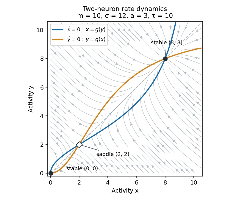
The origin and upper diagonal state attract nearby trajectories, while the lower positive state is a saddle. Its stable manifold separates the two attracting regions: trajectories in each basin of attraction approach its stable node, giving bistability. The diagonal is invariant, and on it the scalar activity increases between $z_{-}$ and $z_{+}$ and decreases between zero and $z_{-}$ or above $z_{+}$. Activities remain nonnegative and bounded because $0\le g\le m$. The vector field has constant negative divergence $-2/\tau$, so the Bendixson-Dulac criterion also rules out periodic orbits in the physical quadrant. The network is a switch between persistent activity levels, rather than an oscillator.

The Jacobian matrix at a diagonal steady state isIts eigenvectors $(1,1)$ and $(1,-1)$ represent common and opposing perturbations, with respective eigenvalues $(-1+g^{\prime })/\tau$ and $(-1-g^{\prime })/\tau$.

For a nonzero equilibrium, ${\sigma }^2+a^2{z}^2=m{a}^{2}z$ and ${\sigma }^2/a^2=z(m-z)$. Consequently $g^{\prime }(z)=2(m-z)/m$. The lower root has $g^{\prime }>1$ and is a saddle equilibrium; the upper root has $0<g^{\prime }<1$ and is a stable node. At the origin $g^{\prime }(0)=0$, so both eigenvalues are $-1/\tau$.

The supplied parameters give $\sigma /a=4$, and the nonzero roots solve $z^2-10z+16=0$, giving $2$ and $8$. The numerical stability results areBiologically, the origin is a quiescent state and the upper equilibrium a sustained mutually reinforced activity state. The saddle represents a collective activation threshold: a perturbation crossing its basin boundary can switch the network from low to high activity. This persistent-state mechanism can model a memory or decision variable, but the simplified rate equations do not establish that a particular biological circuit uses it.

A standard binary Hopfield network contains $M$ recurrently connected units with activities $x_i\in \{-1,+1\}$. Choose symmetric weights $w_{ij}=w_{ji}$, omit self-couplings by setting $w_{ii}=0$, and use zero thresholds for the energy in the next part. To store desired binary patterns ${\xi }^{\mu }$, a simple choice is Hebbian memory weights for a Hopfield network:Correlated activity strengthens connections between units agreeing across the training patterns and makes disagreement contribute negatively. This creates attraction toward the stored configurations when cross-talk is sufficiently small. For one stored pattern, its local field is $(M-1){\xi }_i/M$, so every bit is stable for $M>1$. With multiple patterns, the other patterns add cross-talk; the rule does not guarantee exact retrieval for an arbitrary collection.

Start retrieval from a partial or corrupted cue and update one unit at a time using its current fieldA cyclic or random fair asynchronous schedule lets the network relax toward a fixed point, completing a memory when the cue lies in its basin. This is content-addressable retrieval: the initial pattern selects the memory without an explicit address. Nonzero thresholds can be included in a more general model, but their corresponding linear terms must then be included in the energy.

For the symmetric zero-diagonal weights and asynchronous rule just specified, update only unit $k$. In the energy difference, terms involving neither $k$ nor its symmetric partner cancel. Thus asynchronous Hopfield energy descent givesIf the unit was already aligned, it does not change and $\Delta E=0$. If it flips into alignment, $x_k^{\prime }-x_k=2\mathrm{sgn}(h_k)$, soAt $h_k=0$ our tie rule retains the old activity. The network has only $2^M$ configurations. Strict descent on every actual change prevents revisiting a configuration and permits only finitely many changes. With a fair schedule every misaligned unit is eventually updated, so the terminal configuration is a fixed point. At that point each possible single-bit flip has energy cost $2x_k{h}_k\ge 0$. The network reaches a minimum against single-unit changes, not necessarily the global minimum. Its energy is a Lyapunov function for these asynchronous dynamics.

The qualifications are essential to the printed claim. Synchronous updates can cycle: for two units with $w_{12}=w_{21}=1$, the state $(1,-1)$ alternates with $(-1,1)$, keeping energy $+1$. Symmetry alone therefore does not prove convergence under simultaneous updates.

Nor does the valid descent proof guarantee a global minimum. Consider four units with $w_{12}=w_{34}=3$ and all four cross-group weights equal to $1$, symmetrically and with zero diagonal. The state $(1,1,-1,-1)$ has aligned fields $(1,1,-1,-1)$ and energy $-2$, so it is a strict single-flip local minimum. The all-positive state has energy $-10$. This explicit counterexample shows why local minima may trap retrieval even though the energy always descends under the stipulated rule.

One limitation is finite useful storage capacity and interference. Under simple Hebbian learning, each additional pattern contributes cross-talk to the retrieval fields; correlated or excessive patterns can erase a memory's basin or destabilize the pattern itself. More structured learning can reduce this interference: covariance-based weights account for activity biases, and pseudoinverse-based rules can orthogonalize a set of linearly independent patterns. Sparse representations and suitable thresholds can also change the capacity tradeoff. These extensions require their own retrieval analysis; they do not permit unlimited robust storage in a finite network.

A second limitation is spurious attractors and entrapment in unintended local minima. Mixtures of memories or unrelated configurations can be fixed points, and deterministic energy descent cannot escape an already stable incorrect state. Stochastic updates that sometimes accept energy increases can explore other configurations, and simulated annealing can gradually reduce that randomness to favor lower energies. Better weight learning and basin shaping can reduce the spurious states. Finite-temperature escape is probabilistic, and a practical finite-time annealing schedule does not guarantee the desired memory or a global minimum.

Changing the learning rule addresses interference; changing the retrieval dynamics can address trapping. The objective must still be appropriate: the lowest energy pattern is not necessarily the memory best matching a particular noisy cue.