Simulated annealing accepts worse feasible solutions to escape a local minimum. Minimize an objective function , analogous to energy. Effective temperature has the same units as , absorbing the Boltzmann constant; it controls exploration, rather than a material's thermodynamic temperature.[ref]
Optimization by Simulated Annealing by Scott Kirkpatrick and others. Printed pp. 672–673: effective temperature and cost as energy
Given current feasible point , draw from a proposal distribution . For a symmetric proposal distribution, , use the Metropolis–Hastings acceptance probabilityAccept with this conditional probability; on rejection retain . Every downhill or equal-cost proposal is accepted. Draw a fresh uniform random variable on and accept if . The off-diagonal transition probability includes proposing .[ref]
Optimization by Simulated Annealing by Scott Kirkpatrick and others. Printed p. 672: acceptance rule and rejected proposals
For a maximization problem with objective function , set : every improving proposed neighbor is accepted, and a worsening move of loss has conditional probability of acceptance, under the same symmetry assumption. Likelihood-power annealing uses precisely this sign convention for a log-likelihood. Retain the best feasible solution seen, since the current state can worsen even after a global minimum has been visited.
If the proposal distribution is asymmetric, use the full Metropolis–Hastings acceptance probability, for ,A missing reverse proposal gives zero acceptance. Even a downhill proposal need not be accepted with probability one in this case. Choosing uniformly among a variable number of neighbors is generally asymmetric: and give the correction , where is vertex degree.[ref]
The useful idea is to separate exploring from insisting on improvement: an uphill move can open a route to a better feasible solution. Its usefulness depends on the proposal distribution, the scale of the objective function, and the cooling schedule for simulated annealing. Finite practical schedules carry no general guarantee of finding a global minimum.
To maximize a log-likelihood, use energy and Boltzmann distribution proportional to at temperature . Reversing this sign favors likelihood minima and can make the probability density function nonnormalizable. For Poisson observations with total and sample size , with respect to the normalized probability density function isIts mean is and variance , so it concentrates at the maximum-likelihood estimate as . Cooling of equilibrium laws and convergence of a particular changing-temperature chain are different statements; the latter requires mixing or a direct chain argument.
For independent binomial distribution observations with fixed trial count and total successes , the likelihood-power probability density function relative to is . Its normalized law is the displayed beta distribution. Its mean tends to and its variance tends to zero as , including endpoint maxima. Energy for maximizing a log-likelihood is its negative; the opposite sign reverses the optimization.
Let and . With Lebesgue base measure for , the likelihood-power law has conditionalsThe joint law is proper for , since its marginal is inverse-gamma distribution with shape and scale . There is also a direct convergence proof for successive Gibbs sampling updates with deterministic and . Update from , then from . Inverse-gamma distribution moments and conditional normal moments giveThe coefficients of the preceding moments are bounded by and , so these moments stay bounded from a finite deterministic initial variance. Letting gives and . Also . Thus the iterates converge in mean square to the normal maximum-likelihood estimate.
Consider the chosen finite minimization problemOnly adjacent integers are neighbors. At each interior state propose left or right with probability each; at an endpoint propose its sole neighbor with probability and itself with probability . This proposal distribution is symmetric, including at the endpoints. The local minimum at is relative to these allowed moves; is the unique global minimum.
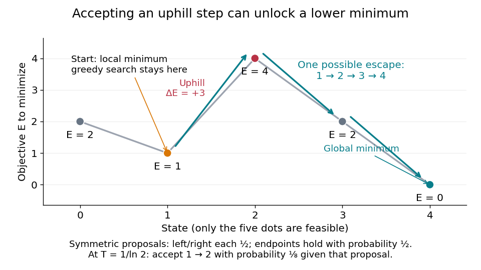
At , improving-only local search rejects both neighbors because and exceed . For simulated annealing, choose , using the natural logarithm. Conditional on proposing from , the acceptance probability isThe one-step transition probability is instead . Both subsequent rightward proposals are downhill, so the conditional probability of the precise next three states being , given and fixed , isThis is one possible escape route, not the probability of eventually reaching . Rejections, excursions toward , and repeated attempts give many other sample paths. The calculation establishes possibility, without claiming a general performance advantage from a selected sample path.
For comparison, halving makes the uphill acceptance probability ; doubling it makes that probability . Cooling makes it harder to leave this local minimum, even though the stationary distribution increasingly favors the global minimum. That tension is the central scheduling problem.
On a finite state space with finite objective function values, the fixed- target is a Boltzmann distribution:The partition function normalizes the weights but cancels from the Metropolis–Hastings acceptance probability. A short detailed balance proof explains the target. With symmetric and ,Summing over gives , so this is a stationary distribution. On a finite state space, a connected graph of positive symmetric proposals makes the accepted Markov chain an irreducible Markov chain. Convergence from any starting state additionally requires an aperiodic Markov chain; one positive self-transition suffices under irreducibility. Replacing by ensures this. For asymmetric , require connectivity through bidirectional proposals: one-way proposals are rejected.[ref]
In the five-state barrier example for simulated annealing, gives exact Boltzmann weights . Multiplying by givesFor the uphill edge, detailed balance is visible numerically:Thus the global minimum has the largest individual stationary probability, , but is far from certain at this positive . At the exact stationary distribution is .
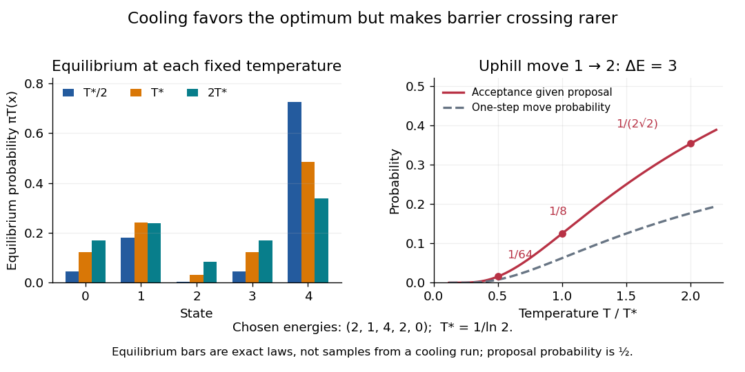
Lower temperature concentrates equilibrium weights while suppressing uphill acceptance
. Exact Boltzmann distributions for the chosen five-state objective function, and the uphill acceptance probability conditional on the proposal . The one-step transition probability is half that acceptance probability. The bars describe equilibrium at each fixed temperature, not the evolving probability distribution during cooling. Details.For any finite , let be the set of global minima and the smallest objective function value. Cancelling from numerator and denominator shows that each nonminimal state's weight tends to zero as , while every state in has equal weight. Therefore tends to the uniform distribution on . This is a statement about a family of equilibrium probability distributions; it does not prove that a cooling Markov chain follows that family.
A cooling schedule for simulated annealing specifies successive effective temperatures and how many proposals to attempt at each. For example, with , using the geometric sequence, can define stages of equal chosen length. Changing changes the transition matrix: if the state probability distribution is , then , which generally differs from . Time spent at one temperature must be compared with its mixing time before equilibrium intuition is justified.
In the five-state barrier example for simulated annealing, fixed gives a finite irreducible Markov chain, so is eventually visited with probability one. That unbounded-time statement gives no fixed finite deadline. Over any finite number of trials starting at , the probability of staying at throughout isEach factor is the rejection probability at . This is an explicit failure event even when every is positive: the best visited objective function value remains , above the global minimum value . More exploratory proposals can help cross a barrier; cooling before those moves occur can preserve a poor local minimum. Successful asymptotic schedules need additional analysis of the allowed moves and barriers.
Historically, Scott Kirkpatrick, Charles Daniel Gelatt Jr. and Mario P. Vecchi connected statistical mechanics with mathematical optimization in 1983. They adapted the Metropolis–Hastings algorithm to cooling searches with symmetric proposals and illustrated computer-design problems.[ref]
Optimization by Simulated Annealing by Scott Kirkpatrick and others. Printed pp. 672–673 and 675: Metropolis procedure, cooling schedule, logic partitioning
Articles by others on the same topic



Simulated annealing is a probabilistic optimization algorithm inspired by the annealing process in metallurgy, where controlled cooling of materials leads to a more stable crystal structure. It is used to find an approximate solution to optimization problems, especially those that are discrete or combinatorial in nature. ### Key Concepts: 1. **Metaphor of Annealing**: In metallurgy, when a metal is heated and then gradually cooled, it allows the atoms to settle into a more organized and low-energy state.