Past exam of the mathematics course of the University of Cambridge / 2008 / iii / Paper 73 / 3

The neutral-hydrogen column density is $N_{\mathrm{HI}}=\int n_{\mathrm{HI}}d\ell$, with units ${\mathrm{cm}}^{-2}$. Define the neutral-hydrogen column-density distribution byHere $\mathcal{N}$ counts absorption systems along a quasar sightline. A histogram per logarithmic column interval instead measures $N\ln (10)f(N,z)$; forgetting this factor changes the inferred slope. Another common convention uses the absorption distance $X$, with $dX/dz=H_0(1+z{)}^2/H(z)$, and $f_X=f/(dX/dz)$.

At a fixed epoch, weak Lyman-alpha forest lines have an approximately falling power-law distribution, $f(N,z)\simeq A(z)N^{-\beta }$ with $\beta \simeq 1.4$–$1.5$ over representative low-column ranges. Stronger absorbers deviate from one universal slope, and the normalization and fitted slopes depend on epoch and sample. The low-column fit is measured, for example, in Kim and collaborators' forest survey. The sketch distinguishes that empirical low-column trend from an illustrative higher-column continuation.

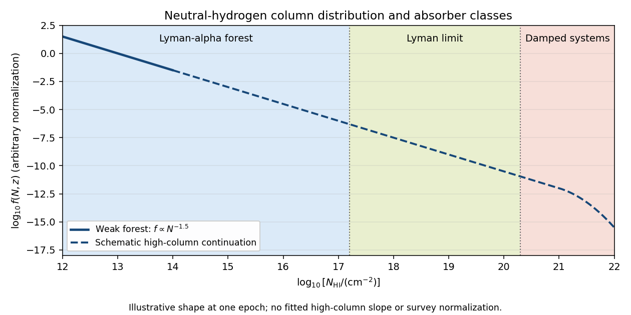
Ordinary Lyman-alpha forest lines cover roughly $10^{12}\lesssim N_{\mathrm{HI}}\lesssim 10^{17.2}{\mathrm{cm}}^{-2}$. They are numerous resonant Lyman-alpha absorption features from intervening gas at different cosmological redshifts, collectively resembling a forest in a quasar spectrum. Many are optically thin at the ionization edge even when their line centers are saturated.

A Lyman limit system becomes optically thick at the $91.2\mathrm{nm}$ hydrogen ionization edge. With ${\sigma }_{912}\simeq 6.3\times 10^{-18}{\mathrm{cm}}^2$, ${\tau }_{912}=N_{\mathrm{HI}}{\sigma }_{912}\gtrsim 1$ requiresIts spectrum consequently has a strong continuum decrement below the redshifted Lyman edge. In a classification separating the highest columns, Lyman limit systems extend up to the damped-system boundary.

A damped Lyman-alpha system conventionally has $N_{\mathrm{HI}}\gtrsim 2\times 10^{20}{\mathrm{cm}}^{-2}$. Its Lyman-alpha absorption is sufficiently strong that the Lorentzian wings of the Voigt profile are prominent. “Damped” refers to the finite radiative lifetime of the atomic excited state, not an inference that the gas has a high temperature. These systems trace substantial neutral reservoirs, usually associated with galaxies.

In the printed convention $\rho$ is energy density, since the gravitational source is $8\pi G\rho /(3c^2)$. For nonrelativistic pressureless matter, ${\rho }_m={\rho }_{m,0}(1+z{)}^3$. Define the cosmological density parameters byThe Friedmann equation then givesLet $n_c$ be the constant comoving number density of absorbers, and let ${\sigma }_p$ be their fixed proper interception area. Their proper number density is $n_p(z)=n_c(1+z{)}^3$, with $a_0=1$. The redshift-time relation gives a local proper photon-path incrementFor an infinitesimal path, the expected number of interceptions, and to first order the probability of an interception, is $d\mathcal{N}=n_p{\sigma }_{p}d\ell$. Thus absorber incidence and comoving number density implyTwo factors survive: proper density brings three powers of $1+z$, whereas proper path length brings the inverse of one power. A fixed comoving area instead of the assumed fixed proper area would change the result. The formula is an incidence rate, not a probability bounded by one over a finite redshift interval; multiple interceptions can occur.

In an Einstein-de Sitter universe, $E(z)=(1+z{)}^{3/2}$. Under the non-evolution assumptions of the previous part, the incidence above a fixed neutral-hydrogen column density threshold consequently scales as $(1+z{)}^{1/2}$. Between the two specified epochs,The higher-redshift rate would be about $41\%$ larger.

Observed Lyman-alpha forest incidence above substantial column thresholds rises much more rapidly. For example, the survey at Kim and collaborators' measurements finds an exponent $2.19\pm 0.27$ for $10^{13.64}\lesssim N_{\mathrm{HI}}\lesssim 10^{16}{\mathrm{cm}}^{-2}$ over this redshift range, giving a representative increase $2^{2.19}\simeq 4.56$, rather than $\sqrt{2}$. The empirical exponent is threshold dependent. The forest therefore cannot be treated as a conserved population of identical fixed-size neutral clouds: gas expansion, structure evolution and the cosmic ionizing background change neutral fractions, absorption strengths and the effective area above the threshold. In photoionization equilibrium, $n_{\mathrm{HI}}\Gamma \simeq \alpha (T)n_e{n}_p$, so changing density or ionization rate changes a counted neutral column even without creating or destroying its baryons.

Use high-resolution quasar spectra to fit Voigt profiles to Lyman-alpha forest lines near $z=3$, where the transition appears near $121.6(1+3)\simeq 486.4\mathrm{nm}$. Each fit estimates the neutral-hydrogen column density and the velocity-width parameter $b$. The one-dimensional Maxwell-Boltzmann velocity distribution has variance $k_{B}T/m_{\mathrm{H}}$; consequently the thermal optical-depth profile is proportional to $\exp [-(v-v_0{)}^2/b^2]$, with the thermal cutoff of Lyman-alpha line widthsFor example, a purely thermal $b=20\mathrm{km}{\mathrm{s}}^{-1}$ corresponds to $T\simeq 2.4\times 10^4\mathrm{K}$.

An observed broad line is not by itself a thermometer: peculiar velocities, bulk gradients, blending and instrumental resolution also broaden it. For independent Gaussian contributions, $b^2=b_{\mathrm{th}}^2+b_{\mathrm{nonthermal}}^2+b_{\mathrm{inst}}^2$. After modeling the instrumental response, an uncorrected total width gives an upper bound on the thermal temperature, not a lower bound. The narrowest lines at each column density are least affected by additional broadening. Their lower envelope in the $b$–$N_{\mathrm{HI}}$ plane constrains the temperature-density relation of photoionized intergalactic gas, often written $T=T_0(1+\delta {)}^{\gamma -1}$.

Calibrate the conversion between column density, density and width with hydrodynamic models incorporating the cosmic ionizing background, pressure smoothing, resolution and selection. It estimates $T_0$ and the slope rather than assigning one temperature to every absorber. Where aligned metal lines trace the same gas, comparing species of different atomic mass can separately estimate a common nonthermal contribution because thermal $b^2$ scales as $m^{-1}$. The forest lower-envelope method and its numerical calibration are developed in Schaye and collaborators' temperature analysis.