A kinematic redshift is the relativistic Doppler effect arising from relative motion of emitter and receiver. In a local inertial frame, recession decreases the received frequency and approach increases it. A cosmological redshift instead compares photons emitted and received by comoving observers at different cosmic times: expansion of the scale factor stretches their wavelengths. It exists even when both observers have zero peculiar velocity. Both are frequency ratios measured by observers, but a large cosmological redshift should not be inserted into a flat-spacetime radial-speed formula to define the galaxy's unique recession speed.
Take for recession. By the definition of kinematic redshift, . Inverting the supplied relativistic Doppler effect and expanding with givesThusA negative radial velocity gives a blueshift at this order.
For a radial null geodesic in FLRW spacetime, the FRW metric gives . The emitter and receiver have fixed comoving coordinates, so two successive wave crests satisfy the same comoving radial distance relation:Subtracting the two expressions in the short-wave-period limit yields . Comoving observers measure these intervals as proper time; since ,For a fixed reception epoch, the cosmological redshift factor is inversely proportional to the emission scale factor. This also shows the associated cosmological time dilation.
In the intended comparison of emission and reception epochs, with negligible peculiar velocities, the Earth-observed cosmological redshifts correspond to and . A photon emitted at the B epoch and received at the A epoch consequently hasThese factors divide, whereas the redshifts themselves do not subtract. There is a geometrical qualification to this usual answer: the two Earth-observed redshifts alone do not specify an arbitrary actual B-to-A observation. The assumed events must be connected by a null geodesic, as when A is on the same radial photon path between B and Earth. If the galaxies have an unspecified angular separation, or A observes at a different cosmic time, the B emission event reaching A is different and its redshift is not determined by these two numbers alone.
The combined kinematic and cosmological redshift is most cleanly found by passing through the emitter's local comoving frame. The distance estimate then requires an explicit approximation to the Hubble law.
Let be the photon frequency in the local comoving frame just after emission. The kinematic redshift gives , and propagation in the FRW metric gives . Multiplication givesEquivalently, . Both redshifts being small is what permits their approximate addition. Here the observer's own peculiar velocity is assumed already corrected to the Hubble flow frame.
In the local, nonrelativistic Hubble law approximation, . Ignoring the peculiar velocity gives an inferred distance , soThe requested accuracy therefore requiresAt exactly the worst-case error is , so “better than” requires a strictly larger distance. This is the conventional leading-order estimate. If one retains the exact Doppler factor and the product term while treating as exact, the positive-velocity case gives , with . It requires . That small refinement is conditional on the distance-redshift prescription; the simple answer uses the local approximation consistently.
For Planck law expressed per unit frequency, put . At fixed temperature, the frequency dependence is . Differentiation givesThe positive interior maximum therefore satisfies , with independent of temperature. The zero solution of the rearranged equation is a boundary, not the interior maximum. Hence the frequency form of Wien's displacement law isThis frequency peak is not divided by the peak wavelength of : the two spectral densities differ by the frequency-to-wavelength Jacobian.
Motion toward incoming cosmic microwave background radiation produces a blueshift. The photon occupation function of a blackbody depends on , so the same Doppler factor multiplies both frequency and effective temperature. Looking forward along the Sun's peculiar velocity, one obtainsTaking the mean cosmic microwave background temperature as about givesThe numerical total inherits the rounded mean temperature; the robust estimate is the positive millikelvin dipole increment.
A K correction accounts for observing a redshifted spectrum through a fixed photometric passband, rather than the corresponding emitted band. In the same R-band astronomical magnitude convention,The luminosity distance already incorporates bolometric dimming; the additional correction depends on spectral shape and band response. At , observed R-band light at was emitted at , in the far ultraviolet. It is not a direct measurement of rest-frame R-band luminosity.
To fix the sign, let be emitted spectral luminosity and approximate R as narrow. Counting photon energy, arrival time and the transformed frequency interval gives . ThusFor an ordinary old elliptical galaxy, the far-ultraviolet spectrum is weak relative to the optical, so typically . Then : neglecting it overestimates the numerical absolute magnitude and underestimates the R-band luminosity. For a young, unobscured star-forming galaxy, hot stars make the far-ultraviolet strong, with an approximately flat spectrum often serving as a useful model. It gives : neglecting it underestimates the numerical absolute magnitude and overestimates the R-band luminosity. Strong dust extinction or an unusual spectrum can reverse this latter sign; a galaxy label alone does not prove an exact correction. The band-integrated convention is given in Hogg and collaborators' definition of the K-correction.
Divide the Friedmann equation by and use . The Hubble parameter therefore satisfiesThe positive root describes the expanding branch. Spatial flatness and the neglect of radiation in cosmology imply .
The age of an FLRW universe at an epoch is the elapsed cosmic time since the Big Bang, not the lookback time from today. For positive matter and positive cosmological constant, integrating givesPut ; then . The integral becomes the age of a flat matter-Lambda universe:Choose such that . The upper-limit value of is , andConsequentlyThe integration constant is fixed by as , where . Equivalently, differentiating changes the last integral to , recovering the supplied trigonometric identity. The formula assumes positive and ; its zero-vacuum limit is regular even though this parametrization is singular.
At , spatial flatness gives , hence and . ThereforeFor , in the previous integral gives , the Einstein-de Sitter universe result. For , the positive-vacuum flat slicing has no finite-age Big Bang, explaining the other endpoint divergence.
In an Einstein-de Sitter universe, , so direct integration of gives . At , and . The fraction of the present age of an FLRW universe and the available formation interval are thereforeThis is only about of the present age. The available interval is itself, not , which would instead be the lookback time.
For and , at the same Hubble constant, the exact integral givesThus the formation interval is longer, by about a factor of . There is also a direct comparison: for , , so is smaller than its Einstein-de Sitter universe value at fixed , and integrating gives a greater age. At the leading matter-era result is ; the smaller matter density, with the same , explains nearly all the increase.
The neutral-hydrogen column density is , with units . Define the neutral-hydrogen column-density distribution byHere counts absorption systems along a quasar sightline. A histogram per logarithmic column interval instead measures ; forgetting this factor changes the inferred slope. Another common convention uses the absorption distance , with , and .
At a fixed epoch, weak Lyman-alpha forest lines have an approximately falling power-law distribution, with – over representative low-column ranges. Stronger absorbers deviate from one universal slope, and the normalization and fitted slopes depend on epoch and sample. The low-column fit is measured, for example, in Kim and collaborators' forest survey. The sketch distinguishes that empirical low-column trend from an illustrative higher-column continuation.
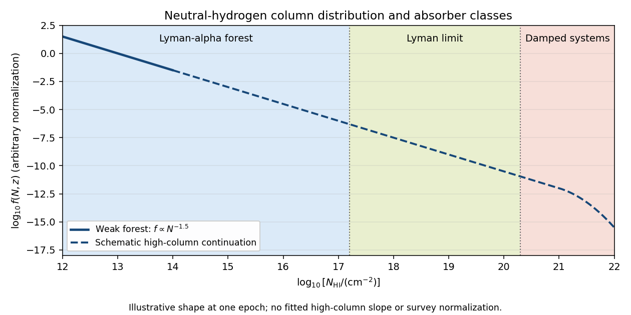

Ordinary Lyman-alpha forest lines cover roughly . They are numerous resonant Lyman-alpha absorption features from intervening gas at different cosmological redshifts, collectively resembling a forest in a quasar spectrum. Many are optically thin at the ionization edge even when their line centers are saturated.
A Lyman limit system becomes optically thick at the hydrogen ionization edge. With , requiresIts spectrum consequently has a strong continuum decrement below the redshifted Lyman edge. In a classification separating the highest columns, Lyman limit systems extend up to the damped-system boundary.
A damped Lyman-alpha system conventionally has . Its Lyman-alpha absorption is sufficiently strong that the Lorentzian wings of the Voigt profile are prominent. “Damped” refers to the finite radiative lifetime of the atomic excited state, not an inference that the gas has a high temperature. These systems trace substantial neutral reservoirs, usually associated with galaxies.
In the printed convention is energy density, since the gravitational source is . For nonrelativistic pressureless matter, . Define the cosmological density parameters byThe Friedmann equation then givesLet be the constant comoving number density of absorbers, and let be their fixed proper interception area. Their proper number density is , with . The redshift-time relation gives a local proper photon-path incrementFor an infinitesimal path, the expected number of interceptions, and to first order the probability of an interception, is . Thus absorber incidence and comoving number density implyTwo factors survive: proper density brings three powers of , whereas proper path length brings the inverse of one power. A fixed comoving area instead of the assumed fixed proper area would change the result. The formula is an incidence rate, not a probability bounded by one over a finite redshift interval; multiple interceptions can occur.
In an Einstein-de Sitter universe, . Under the non-evolution assumptions of the previous part, the incidence above a fixed neutral-hydrogen column density threshold consequently scales as . Between the two specified epochs,The higher-redshift rate would be about larger.
Observed Lyman-alpha forest incidence above substantial column thresholds rises much more rapidly. For example, the survey at Kim and collaborators' measurements finds an exponent for over this redshift range, giving a representative increase , rather than . The empirical exponent is threshold dependent. The forest therefore cannot be treated as a conserved population of identical fixed-size neutral clouds: gas expansion, structure evolution and the cosmic ionizing background change neutral fractions, absorption strengths and the effective area above the threshold. In photoionization equilibrium, , so changing density or ionization rate changes a counted neutral column even without creating or destroying its baryons.
Use high-resolution quasar spectra to fit Voigt profiles to Lyman-alpha forest lines near , where the transition appears near . Each fit estimates the neutral-hydrogen column density and the velocity-width parameter . The one-dimensional Maxwell-Boltzmann velocity distribution has variance ; consequently the thermal optical-depth profile is proportional to , with the thermal cutoff of Lyman-alpha line widthsFor example, a purely thermal corresponds to .
An observed broad line is not by itself a thermometer: peculiar velocities, bulk gradients, blending and instrumental resolution also broaden it. For independent Gaussian contributions, . After modeling the instrumental response, an uncorrected total width gives an upper bound on the thermal temperature, not a lower bound. The narrowest lines at each column density are least affected by additional broadening. Their lower envelope in the – plane constrains the temperature-density relation of photoionized intergalactic gas, often written .
Calibrate the conversion between column density, density and width with hydrodynamic models incorporating the cosmic ionizing background, pressure smoothing, resolution and selection. It estimates and the slope rather than assigning one temperature to every absorber. Where aligned metal lines trace the same gas, comparing species of different atomic mass can separately estimate a common nonthermal contribution because thermal scales as . The forest lower-envelope method and its numerical calibration are developed in Schaye and collaborators' temperature analysis.
Let and count the available neutrons and protons immediately before their incorporation into nuclei. In the usual neutron-limited helium synthesis approximation, all surviving neutrons go into and the remaining protons form . Each helium nucleus contains two neutrons and two protons, soUsing the equal-nucleon-mass approximation and neglecting trace nuclei and binding-energy corrections, the primordial helium mass fraction isThe ratio is the pre-assembly nucleon ratio, not the number ratio of free hydrogen nuclei to helium nuclei afterward. The derivation assumes enough protons to bind all the neutrons, as in standard Big Bang nucleosynthesis. The familiar gives and hydrogen mass fraction .
Under the usual interpretation that the extra force simply slows otherwise adiabatic expansion, without changing reaction rates or injecting particles, the primordial hydrogen mass fraction would be larger. A smaller Hubble parameter makes cooling slower, delays the end of the deuterium bottleneck, and permits more free-neutron decay after freeze-out before nuclear assembly. If the reduced expansion also keeps weak conversions effective longer, the lower eventual cosmological weak freeze-out temperature further reduces the neutron-to-proton ratio. Both effects lower the primordial helium mass fraction and raise the remaining hydrogen mass fraction.
For fixed initial neutron fraction , the post-freeze-out estimate is , where is the onset of efficient nuclear assembly. Thus decreases when cooling delays . The extra time is the time to reach the nuclear-assembly temperature, not an increase in the specified clock interval seconds. An unspecified force that also reheats the plasma, changes weak rates or causes recollapse would require additional information; the simple expansion-only interpretation is essential to this expectation.
A primordial light-element abundance determination seeks gas or stars with little subsequent chemical processing. The three abundances require different observations and corrections.
For helium, measure helium and hydrogen recombination emission in metal-poor extragalactic ionized regions. Correct line ratios for electron temperature, density, extinction, collisional excitation, underlying stellar absorption and unobserved ionization stages. Convert the number ratio to helium mass fraction , allowing for heavy elements when necessary. Since stars produce helium and metals, extrapolate a sample toward zero gas-phase metallicity to infer . The sensitivity to atomic data and these corrections is illustrated by Peimbert and collaborators' helium determination.
For deuterium, fit isotope-shifted hydrogen and deuterium absorption lines in relatively simple, metal-poor quasar absorption systems. The deuterium feature is displaced by about from the corresponding hydrogen line. Multiple transitions and velocity components help distinguish deuterium from unrelated hydrogen contamination. The fitted neutral-column ratio estimates D/H in predominantly neutral gas. Since stellar processing destroys deuterium, low-metallicity, minimally processed absorbers are favored; the technique is exemplified by Pettini and collaborators' deuterium measurement.
For lithium, measure the absorption feature near in warm, old, metal-poor halo stars. Stellar-atmosphere models convert line strength to Li/H. The Spite plateau supplies a nearly constant low-metallicity level, but stellar metallicity trends, atmospheric temperature scales, departures from local thermal equilibrium and stellar lithium depletion must be considered. Thus the photospheric level is not automatically the initial abundance. Ryan and collaborators' halo lithium measurements illustrate the measured abundance and chemical-evolution corrections.
In standard Big Bang nucleosynthesis, with the radiation content and reaction rates fixed, the main adjustable abundance parameter is the baryon-to-photon ratio . The baryon-density consistency between nucleosynthesis and the microwave background usesIncreasing cosmological baryon density makes deuterium burn more efficiently, so D/H falls steeply. The primordial helium mass fraction grows only slowly, because its dominant control is the surviving neutron fraction. Near the observationally favored density, lithium-7 production, much of it initially as beryllium-7, rises with density. At lower densities the full lithium curve has a valley; the sketch focuses on the branch relevant to the baryon-density comparison.
For the historical meaning of “current” in this 2008 paper, representative 2007–2008 fits near areThese local fits, with nuclear-rate uncertainties, and representative D/H and lithium ranges are documented in Steigman's 2007 nucleosynthesis analysis. They are not a replacement for a nuclear network outside their calibrated range.
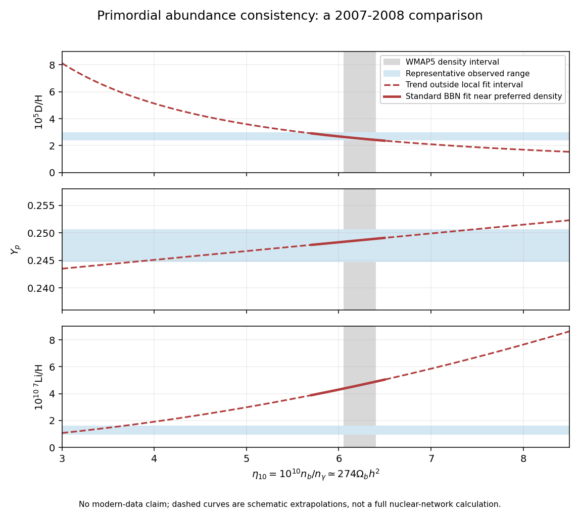
2007–2008 primordial abundance trends and observational ranges compared with the WMAP baryon density
. Details. 
The cosmic microwave background acoustic peak pattern measures baryon loading at recombination, independently of the abundance measurements. For example, the five-year WMAP cosmological analysis gives from WMAP alone, corresponding to . For , this is . Galaxy-cluster baryon fractions combined with independent total-matter density provide another, more astrophysically model-dependent cross-check.
At , the fitted predictions are D/H , , and . A representative observed D/H range around overlaps the prediction; its inferred density is compatible with the cosmic microwave background. The helium result from the 2007 helium analysis also agrees. Other helium analyses had lower central values, illustrating why ionization and temperature systematics matter.
In contrast, a representative plateau estimate corresponds to roughly –, a factor of several below the prediction at the same density. This is the cosmological lithium problem. The three abundance ranges therefore should not all be described as exact simultaneous agreement: deuterium and helium broadly support the independently measured baryon density, while lithium has a substantial discrepancy. The plotted ranges explicitly refer to the 2007–2008 comparison, not present-day parameter estimates.
The agreement of the main light-element abundances with a hot early nuclear-burning phase, and the independent baryon-density consistency between nucleosynthesis and the microwave background, gives strong support to the hot Big Bang framework. These measurements connect the first minutes to recombination, despite their very different temperatures, densities and observables. In particular, the large primordial helium mass fraction and residual deuterium are natural outputs of Big Bang nucleosynthesis, rather than arbitrary products of subsequent star formation.
The cosmological lithium problem prevents claiming that the simplest abundance calculation explains every observation without qualification. One must distinguish nuclear-rate uncertainties, stellar depletion, atmosphere and abundance systematics, and possible new particle physics. Thus the broad hot Big Bang framework is strongly supported, while lithium tests the completeness of its simplest nucleosynthesis and stellar-abundance interpretation. An unresolved lithium discrepancy alone does not erase the independent successes of deuterium, helium and the cosmic microwave background.
Articles by others on the same topic
There are currently no matching articles.