In the Boussinesq approximation, replace density by a constant reference density in inertia and incompressible flow, retaining the small density departure only in the gravitational force. Write and subtract the resting hydrostatic pressure. The upward buoyancy perturbation acceleration and squared buoyancy frequency areThus stable density stratification has . Let henceforth denote the pressure anomaly divided by . The ideal, nonrotating Boussinesq equations areThe buoyancy equation follows by materially conserving the total buoyancy , where ; it does not assume constant .
For an -periodic flow of period , define . An infinite-domain average with vanishing end contributions works as well. The necessary pressure condition is no mean zonal pressure gradient, : periodic pressure satisfies it, whereas a pressure containing a term proportional to does not. Use incompressible flow to write the zonal momentum equation in conservative form,Averaging its zonal derivative terms yields the exact Reynolds stress relation
For two-dimensional small disturbances about rest, the Linearized Boussinesq equations are , , , and . Differentiate the two momentum equations to eliminate pressure: . Differentiating in and using gives . One further time derivative givesThe equation remains valid for . No vertical derivative of was taken: .
For constant and , a plane internal gravity wave hasBoth signs give the prescribed lower-boundary velocity. The radiation condition excludes energy arriving from infinity. At positive frequency, the vertical group velocity isFor a source below the fluid, energy must propagate upward, so the outgoing solution has , even though its vertical phase velocity is downward.
To obtain this selection causally, let and , and replace the constant amplitude by . The method of multiple scales treats as independent during differentiation: the carrier derivatives hold fixed, while holds fixed and holds fixed. Only after differentiating do we restrict to , . Acting on the complex wave, the operators becomeWith , the wave equation has residualThe zeroth-order term is the dispersion relation; the first-order term vanishes precisely whenIf is the switched-on boundary amplitude, with for , the outgoing envelope is for . Its characteristics carry the boundary signal into initially undisturbed fluid. If , characteristics instead arrive from the upper half-space; zero initial disturbances and no incoming signal cannot establish the proposed boundary-forced wavetrain. This is the internal-wave envelope radiation condition.
The leading incompressible flow polarization gives . Hence, to second order in amplitude and leading order in the slow modulation,There is no meridional transport here. Envelope transport gives , so an initially vanishing mean develops asThese are the leading expressions for internal-wave momentum deposition; higher slow-modulation corrections to the stress are beyond the displayed approximation. In particular, a spatially uniform fully established wavetrain has zero stress divergence, but the front has already produced its mean flow.
The mean wave energy density per unit mass follows from :Thus . In the original frame the mean kinetic energy is . In a frame translating at , the undisturbed velocity is , and the change in mean kinetic energy is . Indeed at this order behind the front. Mean-flow energy is therefore essential at the same order as wave energy in the translating frame. This follows also from the frame transformation of energy, up to the fixed background constant, and is why conservation of momentum cannot be omitted from the moving-frame conservation of energy budget.
A precise stratification–rotation analogy uses constant , ideal fluid, and independence of one horizontal coordinate. For the stratified system take , , and allow prescribed forces . The possibly nonlinear Boussinesq equations areFor the unstratified system choose right-handed coordinates , rotation , and . Its rotating Euler equations, with the static gravitational and centrifugal contributions absorbed into the background pressure, arewhere . The identification isThen , , and , proving the component-by-component equivalence. In particular, buoyancy perturbation maps to transverse rotating velocity, and stratified horizontal velocity maps to rotation-axis velocity. The mapping permits arbitrary prescribed forces in the two-dimensional plane, but no transverse force: a transverse force in the rotating problem would create a source in the stratified buoyancy equation. A transverse stratified force would also invalidate . Constant is essential to this constant-rotation equivalence.
A physical free surface introduces extra structure beyond the interior equations. After subtracting hydrostatic pressure, its zero total pressure condition gives to first order, together with the kinematic condition for the stratified vertical displacement. The mapping takes this normal velocity into , whereas an actual rotating free surface normal to its physical vertical has normal velocity and a displacement along . The image of the stratified horizontal surface is a vertical surface in the rotating coordinates. Consequently the physical free-surface problems are not analogous, although deliberately mapped rigid boundaries or mathematical boundary data can be.
For the first prescribed force, the steady linear stratified equations are satisfied byReal parts are understood. The horizontal pressure gradient balances the force; the vertical pressure gradient is balanced by buoyancy; and satisfies buoyancy conservation and incompressible flow. Thus neither nor is fixed by the steady equations alone.
Initial rest and switching on in the unbounded fluid remove this ambiguity by causal pressure adjustment by internal waves. Work with the coefficient and let be the horizontal Fourier transform of . For an abrupt switch at time zero, elimination in the linear equations givesAt the bracket cancels the apparent singularity at every finite time. The persistent pressure term is the symmetric antiderivative of the force: the inverse transform of , interpreted as a Cauchy principal value, is . The oscillatory part propagates away. To see why its zero-frequency part does not leave an arbitrary offset, note that with ; its long-wave contribution consists of oppositely moving fronts. At fixed , the two far-field values of are and , whose average is zero. Nonzero horizontal wavenumbers give dispersive transients that decay locally. Smooth finite-duration switching changes the transient, not this selected steady limit. ThereforeA spatially constant pressure gauge is immaterial. The long-wave group velocity gives the adjustment scale: the elapsed time since switching must satisfy and , and exceed the switching duration. These are asymptotic conditions, not an assertion of exact equilibration after a finite time; the full dispersion relation allows tails. The same long-wave limit gives if desired. Equal-amplitude outward fronts leave opposite pressure offsets and the same velocity on their two sides.
For the force depending instead on , any steady linear horizontal momentum balance requires and . Their mixed derivatives disagree wherever , since but . Hence no steady linear velocity field can satisfy the equations, irrespective of whether it is -independent. This statement concerns the linearized problem; nonlinear inertial balances were excluded by the assumptions.
For an unsteady solution put and take . Its horizontal divergence is zero. The pressure derivatives needed in momentum balance areTheir compatibility is exactlyThus the Poisson equation supplies an actual pressure and the proposed velocity solves both momentum equations; the vertical momentum and buoyancy equations hold because . This flow grows linearly in time, so it remains a valid small-disturbance prediction only while its velocities are small.
As with total force fixed, . Set . Away from the source , and decay at both ends requires . Integrating across the source gives the jump . Since this jump is , , soThis verifies the distributional source as well as the decay condition.
The corresponding rotating problem is not expected to reproduce this evanescent accelerating flow. Its forcing varies in , precisely the coordinate whose independence was required in the stratification–rotation analogy. Moreover, maps to the rotation-axis coordinate . At small Rossby number, the Taylor–Proudman theorem gives in the unforced exterior regions. Such nonzero columns cannot decay with , hence cannot reproduce an tail. There is also a direct unsteady obstruction to copying the proposed flow: in a homogeneous fluid rotating about the mapped axis, a mode with nonzero axial wavenumber has inertial wave frequency of magnitude , rather than the zero-frequency horizontal vortical response of the stratified problem. The steady or slowly varying exterior rotating response must be columnar or accompanied by outgoing inertial waves; the decaying stratified solution is outside the partial analogy.
Let denote free-surface height and the water depth. The inviscid rotating shallow water equations with constant Coriolis parameter areIt is , not , that supplies the horizontal pressure gradient. For a fixed bottom, mass conservation equivalently gives .
Write for relative vorticity. Differentiate the second momentum equation in and the first in , then subtract. The pressure terms cancel. Expanding the differentiated advection terms givesConsequently the absolute vorticity satisfies . Combining this with mass conservation yields exact shallow-water potential vorticity conservation:A sloping bottom changes the depth and hence the stretching, but contributes no curl to the gravitational pressure force.
For the quasi-geostrophic approximation, choose constant reference depth , speed , and horizontal length . Require Rossby number , slow evolution on the advective time , smooth horizontal scales, and or smaller, where is the Rossby deformation radius. Write , , and . The leading momentum balance is geostrophic balance:It gives , while we require and slopes on the chosen horizontal scale. Relative vorticity divided by is also . ThusThe derivative of the constant first term vanishes. In advecting the first-order anomaly, the ageostrophic flow contributes only at the next order. Therefore the shallow-water quasi-geostrophic potential vorticity equation isThis retains the balanced vortical branch, including Rossby waves driven here by the topographic potential-vorticity gradient. It filters the freely oscillating inertia–gravity branches of the full shallow water equations, and does not retain independent boundary Kelvin wave dynamics. Small Rossby number alone is insufficient for the reduction: fast waves must be absent at leading order, as in well-prepared balanced initial data.
In the channel take and measure the bottom anomaly from mid-channel: . Define . The resting potential vorticity is , and the linear Rossby wave equation isFor nonzero zonal wavenumber , wall conditions selectThe modes are stationary. Write and take real for the following sketch. The total potential vorticity is . For a contour whose undisturbed position is , its small meridional displacement isThus potential-vorticity conservation says a northward displacement in a positive background gradient carries a negative anomaly, . Potential-vorticity inversion turns this into positive and anticyclonic motion around the bulge. At a positive cosine crest, is northward on its western flank and southward on its eastern flank. Advection raises the contour on the west and lowers it on the east, so the crest moves west. Algebraically, and give , the same phase velocity as above. For all propagation directions reverse.
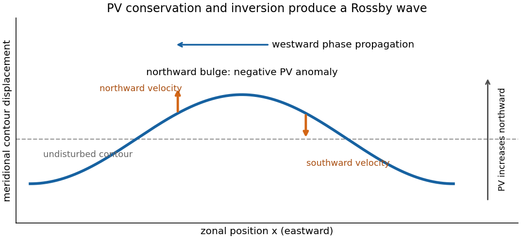
Potential-vorticity contour displacement and westward Rossby-wave propagation for a positive background gradient
. Details. 
For a square basin use a nonzero-frequency normal mode , with on all walls. Its equation isSet and . Substitution cancels the first derivative and givesThe square's Dirichlet Laplacian eigenfunctions are , with positive integers. Consequently the square-basin topographic Rossby mode hasFor , the positive-frequency branch therefore tends to as , as required. The negative-frequency solution is its complex-conjugate representation for a real disturbance; the physical frequency magnitude is .
The geostrophic material derivative isIt advects horizontally with the geostrophic flow. The exact material derivative additionally includes horizontal ageostrophic flow and vertical advection . The leading balances are geostrophic balance and the hydrostatic approximation:The conventional quasi-geostrophic streamfunction is , after fixing the horizontally uniform reference pressure consistently with the basic buoyancy profile. ThereforeHere and below pressure is divided by reference density, and is the anomaly about the prescribed background buoyancy.
For the zonal average assume periodicity or vanishing boundary terms, so that averages of derivatives vanish and averaging commutes with derivatives. Put . Since , the disturbance quasi-geostrophic potential vorticity is . The zonal part of vanishes as . For the other parts, integration by parts givesAs , , and , the Eliassen–Palm flux isWe have therefore proved the exact Taylor identity for quasi-geostrophic flux,without imposing small amplitude. This identity is algebraic within the quasi-geostrophic approximation; it does not assert validity of that approximation for arbitrary physical flows.
Now linearize about a steady zonal basic flow , with and no mean meridional velocity. The linear quasi-geostrophic potential-vorticity equation is . Multiply by and average. The advection term is a zonal derivative and vanishes, givingThis is quasi-geostrophic wave-activity conservation law. The basic-state denominator is time-independent at the retained order; its change caused by the waves is higher order. The wave activity is signed if , and the formula cannot be used where that gradient vanishes. The original PDF includes the zonal average over the squared disturbance in this definition.
For the resonant solution it is helpful to avoid squaring an imaginary coefficient as though it were real. Writewhere is real. Assume , , and . Define and . The complex coefficient of the physical streamfunction disturbance isThe original PDF contains : the converted TeX's missing would incorrectly remove the resonance and fails the differential equations.
For the vertical potential-vorticity inversion operator, and . ConsequentlySubstitution in the linear potential-vorticity equation givessince . Thus this is a genuine resonant topographic quasi-geostrophic wave, with linear amplitude growth rather than an assumed stationary wave.
At the flat upper boundary , so . At the lower boundary, linearization of the impermeability condition gives , where is the bottom corrugation. Here is time-independent, so the specified vertical velocity givesusing . Both boundary conditions are verified. The linear solution is valid while its growing displacement and velocity remain small; it is not a large-time nonlinear solution.
To evaluate all fluxes, use . The coefficients of are respectively , , and . HenceThe products of the terms alone and the terms alone are imaginary in the vertical flux and contribute nothing. Only the cross terms remain. Sincewe obtainDifferentiating gives . As ,For an independent evaluation of the right side of the Taylor identity for quasi-geostrophic flux, write . Multiplication of by gives real part , because the remaining real cross terms cancel. Thereforewhich verifies the flux identity pointwise in .
The basic potential-vorticity gradient is , so the wave activity and its derivative areHere follows from . Thus . The growth term involves ; the distinction matters because the printed complex coefficient is imaginary. These formulas evaluate both flux components, their divergence, the buoyancy and PV covariances, and wave activity. In particular and , so for the growing activity is supplied by the positive flux from the lower boundary.
Finally put and write the height-independent mean velocity change as . Since and can be chosen independent of height, the mean potential vorticity becomesTo be uniform in this requires for some constant . Integrating and applying both endpoint conditions gives , , and hence . ThereforeThe constant is the initial channel-mean potential vorticity, as also follows from . This is the momentum loss from uniform potential-vorticity mixing. Averaging the velocity change across the channel gives the momentum change per unit mass,For positive the mean current is reduced everywhere in the interior. The imposed bottom can exchange momentum with the fluid, so this change is consistent with the complete conservation of momentum budget.
Articles by others on the same topic
There are currently no matching articles.