Write and for the population and empirical measure. The empirical distribution function isFix and a finite cover by function brackets of width below . If belongs to the th bracket, thenand, using instead, . ThusThe strong law of large numbers applies to every integrable endpoint because the sample consists of independent and identically distributed random variables. For this finite collection the maximum tends to zero on a common probability-one event. Apply the argument for , , and intersect those countably many events. On the resulting event the limsup is at most for every , proving the uniform strong law from finite L1 bracketing. This pathwise argument also avoids assuming without justification that an arbitrary uncountable supremum is measurable.
For the Glivenko-Cantelli theorem, take . Here is a finite bracketing construction which also handles atoms of the distribution. Choose and divide the possible values of into finitely many bins , including the final value one. For each nonempty parameter set , set and pointwise. These functions are indicators of rays, possibly with an open endpoint, so they are measurable. Monotonicity of and monotone limits at the extreme thresholds give and . Hence . No continuity of is required. Applying the proved uniform law givesFor an uncountable class of continuous functions, use . The functions are distinct, bounded and integrable for every probability law. Moreover by the strong law of large numbers. This supplies the requested example without additional compactness machinery.
For a normalized kernel for density estimation , with , the kernel density estimator isIt replaces each atom of the empirical measure by a translated, scaled copy of : averaging these small probability-density bumps gives a smooth approximation to the sampling density. Integral one is part of the probability-kernel convention; without it, the estimator generally targets .
The printed bandwidth assumption is insufficient for the claimed normal limit. The additional condition is needed at points with positive density. For a counterexample, take a normal distribution density , , the unit-width box kernel and . Then , but the probability that any observation lies in the window is at most . On the complementary event the estimator is zero, and . The limit in probability is therefore zero, whereas the stated normal limit has positive variance.
We now prove the intended pointwise central limit theorem for a kernel density estimator under , and . The first condition also follows from the last one. A mean value theorem bound, with , gives the bias of a kernel density estimatorThus the bias multiplied by tends to zero.
The Lindeberg-Feller central limit theorem says that independent centered variables in each row of a triangular array have sum converging in distribution to if the sum of their variances tends to and, for every , the sum of their truncated second moments tends to zero. Put and . The independence hypothesis holds within each row. A change of variable givesContinuity of at and the compact support and boundedness of justify the limit. Also , so the Lindeberg condition is eventually identically zero for every . The sum is exactly . Combining the centered limit with the negligible bias by the Slutsky theorem provesIf , the centered variance tends to zero, and the Chebyshev inequality proves the corresponding degenerate limit directly.
For , let be the supplied -quantile of this limiting normal distribution. Inverting the limiting central probability gives the confidence intervalContinuity of the limiting distribution gives asymptotic coverage . Equivalently, its half-width is under the stipulated oracle quantiles. A degenerate limit at does not by itself justify this nominal-coverage normal interval.
Let be the scaling function and an orthonormal wavelet, with and . For , the wavelet series at a coarse level isThe series converges in the L2 norm. Its coarse part captures broad variation and successive wavelet levels add finer detail. Truncating at levels produces the orthogonal projection onto ; Parseval identity makes its squared approximation error the sum of the omitted squared coefficients. Merely square-integrable functions need not have pointwise convergence.
For the Haar wavelet, use the cell convention and let be the unique such interval containing . The Haar scaling functions are , so the Haar projection isFor a merely locally integrable function this cell-average formula remains defined, even if a global orthogonal projection is unavailable. If , the mean value theorem gives Lipschitz continuity and, since on the cell,Thus the requested bound holds with , by the Haar projection error for a Lipschitz function.
To estimate a density, replace each scaling or wavelet coefficient or by the sample average of that basis function. The finite-resolution Haar density estimator is thereforeIt is the histogram on the dyadic cells, is nonnegative, and integrates to one. Its expectation is . A density with bounded derivative is bounded: the Lipschitz density height bound gives by integrating the triangular lower envelope . The case cannot be a probability density on the whole real line. Hence .
The cell probability is . The sample count has a binomial distribution, soThe Cauchy-Schwarz inequality bounds the mean centered absolute deviation by the square root of this variance. Adding the projection bias givesChoose , so . The two terms have the same order, andThis is a bias-variance tradeoff: refining the cells decreases the averaging bias but increases the sampling variance.
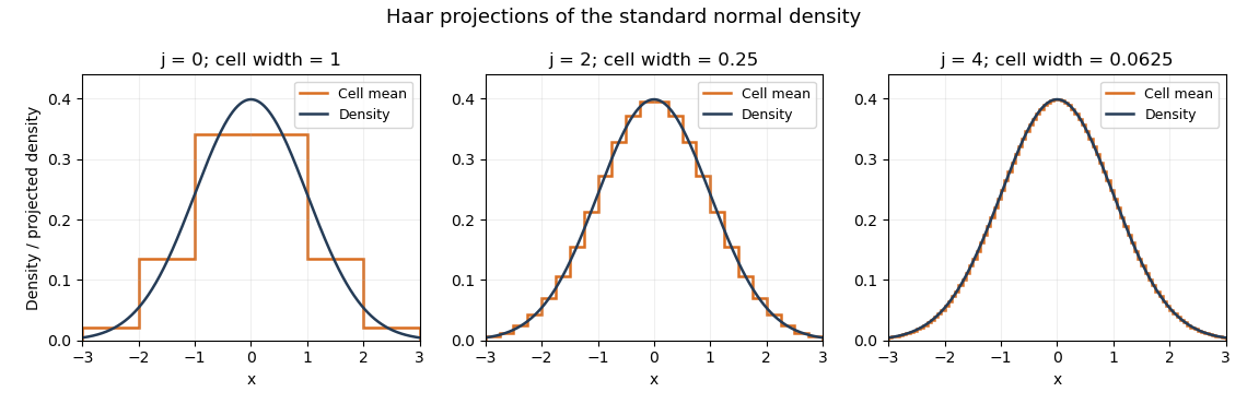
Haar projections of the standard normal density at three resolutions
. Details. 
The Haar projection averages this normal distribution density on each cell; the finer cells follow its variation more closely. A Haar density estimator replaces these exact cell probabilities by empirical frequencies and therefore also introduces sampling noise.
The Nadaraya–Watson estimator isFor the unit-width box kernel, it averages the responses with design points in . Define it to be zero if that window contains no observations; the supplied small-denominator bound must refer to a defined estimator.
Write , and . Set . On ,This is the absolute error bound for a ratio estimator with a controlled denominator; it does not require the numerator and denominator to be independent.
The conditional expectation definition of the regression function givesAt this interior point, the Taylor theorem expansions are and . Multiplying and using the symmetric interval removes the odd linear term. More precisely,This cancellation underlies the interior absolute-error rate of the Nadaraya-Watson estimator.
For the variance, independence between observations givesConditional on , the second moment is . The bounded conditional variance, local boundedness of , and boundedness of consequently make the expectation at most . Thus . By the Cauchy-Schwarz inequality,The auxiliary result supplied in the question makes the expected error on equal to . Combining both events, with , provesBoth the squared-bandwidth bias and the inverse-square-root window-count error have this order. The supplied separate consistency result for the design-density estimator is not needed once the stronger small-denominator expectation bound is used.
Articles by others on the same topic
There are currently no matching articles.