An orthonormal wavelet generates an orthonormal basis of throughThe factor compensates for the shrinking support of a function, keeping the L2 norm equal to one. Orthogonality makes different coefficients separate squared-norm contributions, and completeness allows the wavelet series to recover any square-integrable function in the L2 norm.
For the Haar wavelet, wavelets at one scale have disjoint supports. At different scales their dyadic intervals are either disjoint or nested. On the support of the finer wavelet, the coarser one is constant, while the finer one has zero integral, so their L2 inner product is zero. Together with the unit L2 norm, this explains orthonormality. On the bounded interval , add the constant Haar scaling function and use , ; the constant function is not an basis element on the whole line.
A Daubechies wavelet of order is a compact support orthonormal wavelet with vanishing moments and a minimal-length finite refinement filter. The minimal filter has taps, giving support length in the standard dyadic normalization. Its low-pass symbol has a zero of order at . Increasing order improves polynomial cancellation and, for sufficiently large order, regularity, at the price of a wider support.
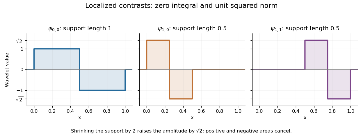
The Haar wavelet is a signed contrast between two adjacent half-intervals:It has compact support, zero integral, and unit L2 norm: and . The zero integral is its one vanishing moment. Its Haar scaling function is , which records a coarse value rather than a contrast. Endpoint conventions do not alter the L2 inner products.
The normalized copies compare the halves of the dyadic interval . Narrower copies are taller so that their L2 norms stay one. Thus a coefficient identifies both a location, through , and a scale, through .

For a simple step function equal to on and on , its coarse coefficient is , while its first contrast is . Thus . The negative coefficient raises the second half and lowers the first. Finer contrasts vanish because is constant on each half. A jump aligned with this dyadic interval boundary therefore needs only two nonzero coefficients; jumps at other positions can require details at many scales.
Its jump discontinuities make the Haar wavelet particularly transparent for changes between neighbouring regions, while limiting approximation of smooth variation. A Daubechies wavelet uses a more elaborate pattern to obtain additional vanishing moments and, at sufficiently high order, smoother basis functions. The elementary Haar refinement identity has coefficients and explains how the coarse and fine descriptions fit together.
The historical source is Alfred Haar's [ref]
https://history-of-approximation-theory.com/fpapers/haar1910.pdf. Zur Theorie der orthogonalen Funktionensysteme, Mathematische Annalen 69 (1910), pp. 331–371
. Chapter III, beginning on page 361, constructs the constant function and these localized piecewise-constant orthogonal functions. Its original endpoint assignments differ from the half-open convention used here, without changing L2 inner products.Use the full orthonormal Haar system, including the constant function. Dyadic partial sums are cell averages and converge uniformly for continuous . On a cell of length , a normalized detail has and pointwise size . Fix a coarse level where the modulus is small. Above a level chosen by reaching that small modulus, no detail can survive the threshold. Below it, omitted details along any one dyadic chain sum to a geometric bound. Thus the thresholded expansion differs from a sufficiently fine cell average by a uniformly small amount.
At each point there is at most one supported Haar wavelet per scale. If a detail coefficient is below , its value there is at most . Summing these bounds up to level gives the displayed geometric estimate. Selecting so the final term is of the order of the modulus of continuity controls all omitted fine details, even though arbitrary deletions from a uniformly convergent series need not preserve convergence.
The normalized Haar scaling functions and wavelets obeyThis orthogonal two-by-two transformation gives the multiresolution analysis decomposition . Iterating it expresses a Haar approximation either through level- cell averages or through coarse averages and all wavelet details at lower levels. The identities remain valid locally for coefficient integrals of locally integrable functions, without a global assumption.
The Haar projection at level is the orthogonal projection onto the functions constant on level- dyadic intervals. On each cell it replaces by its cell average. This is the closest cellwise-constant approximation in the L2 norm, because choosing a constant on a cell minimizes at its cell average.
On , take the step function with values on successive quarter-intervals. At level zero, its Haar projection is the constant . At level one, it has values and on the two halves. At level two, it recovers the four original values exactly. With normalized Haar wavelets, these approximations areThe coefficients are L2 inner products, so they differ from the discrete vector coefficients by the factor . Their squared sum also has a direct meaning:The approximation errors in squared L2 norm of are respectively : each added detail removes exactly its own squared coefficient from the error.
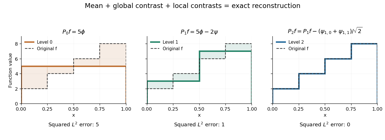
Coarse mean, half-interval contrasts and quarter-interval details reconstruct the same four-step function
. Details. 
The Haar projection can be expressed using level- Haar scaling functions, or through a coarse scaling family and the Haar wavelets at intermediate levels. On with lowest level zero, that coarse family is the single constant function . On the whole real line, use the integer translates of a coarse Haar scaling function instead; one global constant is not square-integrable. Refinement improves the representation while retaining the earlier coefficients.
The Haar projection replaces a function by its mean on each dyadic interval of length . For a function satisfying Lipschitz continuity with constant , every value in a cell differs from its cell mean by at most . This bound holds for all points with a consistent endpoint convention, and requires no global L2 norm assumption when the projection is defined by local averages.
Finite total variation of a function on gives the following error bound for averaging on dyadic cells of length :The cell error is at most its length times the oscillation on that cell, and the sum of the oscillations is at most the total variation. This proves that the difference is integrable even if is not globally in . For an even function decreasing to zero on the positive half-line, and the bound becomes .
In the Gaussian white noise model, estimate a Haar scaling function coefficient by . The resulting Haar projection estimator is an unbiased estimator with independent coefficient errors of variance . On each cell it is the observed path increment divided by the cell length. This gives a finite-dimensional estimator without imposing smoothness on the drift.
The cellwise error of the Haar projection estimator in Gaussian white noise is times a standard normal variable. Its supremum norm is therefore exactly that factor times the Gaussian maximum over cells. The Gaussian maximum bound without independence gives expected error at most . This concerns the stochastic error about the projection; approximation bias must be added when estimating the full drift.
At level , a Haar scaling function is the normalized indicator function of the dyadic interval . Its L2 norm is one because its squared height is and its support length is .
For a real square-integrable function , its coefficient isMultiplying the coefficient by the Haar scaling function restores the cell average on that interval. The disjoint supports make the functions at one level an orthonormal basis of the cellwise-constant subspace. This normalization is also what turns coefficient variances in the Gaussian white noise model into and cellwise variances into in the Haar projection estimator in Gaussian white noise.
Articles by others on the same topic
There are currently no matching articles.