A phase diagram partitions a space of control parameters into regions with distinct equilibrium phases. Its boundaries mark nonanalyticities of the thermodynamic-limit free energy; a first-order phase transition has a jump in a first derivative, whereas a continuous phase transition has a continuously vanishing order parameter and singular fluctuations.
An explicit three-parameter example is the scalar Landau free energywith parameter axes . These can be realized locally by the temperature, single-ion anisotropy and magnetic field of the Blume–Capel model. The three dimensions here refer to control-parameter space, not necessarily to three spatial dimensions. At , minimizing this potential gives a continuous phase transition at for . For , coexistence occurs at , whereThere are three global minima, and . Their order parameter jump decreases to zero as . Thus is a tricritical point. The two transition curves in the plane meet there.
In the three-dimensional phase diagram, crossing inside the ordered region switches between opposite signs of , so that region is itself a first-order phase transition sheet. For , two tricritical wings at opposite nonzero fields separate weakly and strongly magnetized phases. Their wing critical edges can be obtained rather than merely sketched: require . Since , the nonzero solutions satisfyThe fourth derivative there is , giving ordinary continuous critical endpoints. The wings meet the zero-field coexistence sheet along the tricritical three-phase line and terminate at these edges. Their exact tricritical wing coexistence factorization supplies the surfaces in the figure: for two nonnegative minima , set , andDirect expansion gives , proving that these surfaces describe coexistence of global, not merely local, minima.
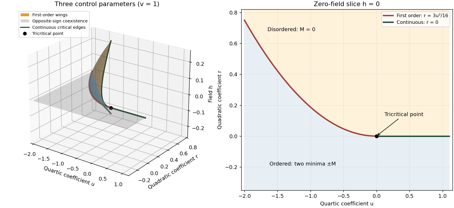
Tricritical phase diagram of the sextic scalar free energy: first-order sheets, critical edges and the zero-field slice
. Details. 
For the unheaded Ising model calculation, assume ferromagnetic exchange and let denote the mean Ising spin. On the hypercubic lattice the coordination number of a lattice is , even though the original positive-direction bond sum counts each bond only once. The mean-field approximation neglects products of deviations from :There are bonds, so the approximate energy is . Each independent Ising spin therefore sees the effective field . With , averaging its two Boltzmann weights gives the self-consistency equationThe slope of its right side at zero is , whereAbove , for excludes a nonzero solution. Below the initial slope exceeds one, and concavity of the hyperbolic tangent on the positive axis gives one positive solution and its negative partner. The Ising auxiliary mean-field free energy has positive quartic coefficient near , while its quadratic coefficient changes sign there. Its stable minima therefore move continuously away from zero; this is a continuous phase transition in the mean-field theory of the Ising model.
Put and . The Taylor expansion gives, on the nonzero branch,Consequently and the mean-field order-parameter exponent is . The inverse-temperature symbol used above is distinct from this order-parameter critical exponent.
For a ferromagnet the scalar order parameter is the spontaneous spin magnetization. It distinguishes a symmetry-invariant phase with zero mean from one of two phases with a nonzero mean of opposite signs. At zero field, a finite system with spin inversion symmetry has exactly zero mean. The spontaneous value is defined by taking the thermodynamic limit first and then sending the symmetry-breaking conjugate field to zero from one side.
A Landau-Ginzburg theory promotes the coarse magnetization to a scalar field and usesAt , spin inversion symmetry permits only even local powers. The gradient term penalizes spatial variations. The equilibrium statistical weight is ; the Landau approximation chooses a stable minimum of , whereas the full functional integral retains fluctuations around it. In a homogeneous phase this gives the equation of state . The field is conjugate to the order parameter, with .
Use the connected correlation function , since the disconnected constant in an ordered phase does not measure fluctuation decay. Away from criticality its large-distance exponential defines the correlation length:when that limit exists. Algebraic prefactors do not affect this definition.
Expand the Landau-Ginzburg theory about a stable homogeneous minimum . With , the quadratic fluctuation energy is . The Gaussian functional integral givesThis Ornstein--Zernike correlation function shows why the curvature of the free-energy minimum controls correlations. At a continuous phase transition that curvature vanishes, allowing long-range fluctuations. In the ordinary quartic theory with , above the transition and on either ordered branch below, so on both sides. At an equilibrium first-order transition the competing minima generally retain nonzero curvature, and the correlation length remains finite. The limit of local stability at a spinodal point is a distinct mean-field phenomenon.
Microscopically different systems can have the same critical exponents and appropriately normalized scaling functions. This universality means that they belong to one universality class when coarse-graining brings them to the same renormalization-group fixed point. Spatial dimension, order parameter symmetry and the range of the interactions affect that classification; changing a lattice spacing or a microscopic coupling generally changes nonuniversal amplitudes and the critical temperature instead.
In the scalar short-range Landau-Ginzburg theory, a positive quartic term and one thermal tuning produce ordinary Ising-type criticality. A generic sextic term does not change that fixed point, but tuning the quartic coefficient to zero exposes a different tricritical point with different exponents. The mean-field approximation itself neglects fluctuations. Its numerical exponents are reliable only when the Ginzburg criterion makes those fluctuations subleading; the ordinary scalar upper critical dimension is four, while the tricritical one is three. At an upper critical dimension logarithmic corrections can remain.
Set in the even sextic Landau free energy. For , near the nonzero stationary branch satisfies for . The minimum value is below the transition and zero above. The order parameter is continuous, and if crosses zero linearly with temperature, the first temperature derivative of the minimized free-energy density is continuous too. There is no latent heat; a second derivative has a finite jump at this level.
For , solve the two conditions and with . Setting gives and . Eliminating givesBoth the disordered and ordered minima have positive curvature there, but their values coincide. Crossing this phase coexistence boundary changes the global minimum discontinuously. The order parameter jumps; for at fixed , jumps as well, generically yielding a nonzero latent heat. Local extrema can persist past coexistence as metastable states, which explains hysteresis in a dynamically delayed transition. The spinodal points, where local curvature vanishes, do not locate the equilibrium transition.
The first-order coexistence curve approaches the continuous curve as : both meet at . To obtain this tricritical point, two even coefficients must be tuned to zero, while the sextic coefficient remains positive. A nonzero conjugate field removes the zero-field inversion symmetry and leads to the wing structure described in the root solution.
At , the equation of state becomes . For ,Above the transition and . These are stable branches of a bounded potential, and the ordered value tends continuously to zero at , but with rather than the ordinary square-root law. Tricritical behavior requires , and ; a generic path with fixed instead has ordinary critical behavior.
A critical exponent is the leading power of a singular observable as a control variable approaches a critical value. Use and distinguish the exponents from coefficient names in a Hamiltonian. Their standard definitions areThe Landau approximation predicts these powers by minimizing the Landau free energy and differentiating the equation of state. At an ordinary quartic point, , above and below, and on the critical isotherm. The equilibrium singular free energy is proportional to below, giving a heat-capacity jump. The quadratic fluctuation denominator is , so and . Thus the ordinary mean-field critical exponents areAt a tuned tricritical point, the preceding solution gives , and below. At the equation of state is . The curvature still vanishes linearly, and the Gaussian gradient term still gives zero anomalous dimension. ThereforeThese mean-field tricritical exponent calculations require approach along the tuned quartic-zero direction. Fluctuations modify the powers below the appropriate upper critical dimension, and marginal effects can add logarithms at it.
Articles by others on the same topic
There are currently no matching articles.