A phase diagram partitions a space of control parameters into regions with distinct equilibrium phases. Its boundaries mark nonanalyticities of the thermodynamic-limit free energy; a first-order phase transition has a jump in a first derivative, whereas a continuous phase transition has a continuously vanishing order parameter and singular fluctuations.
An explicit three-parameter example is the scalar Landau free energywith parameter axes . These can be realized locally by the temperature, single-ion anisotropy and magnetic field of the Blume–Capel model. The three dimensions here refer to control-parameter space, not necessarily to three spatial dimensions. At , minimizing this potential gives a continuous phase transition at for . For , coexistence occurs at , whereThere are three global minima, and . Their order parameter jump decreases to zero as . Thus is a tricritical point. The two transition curves in the plane meet there.
In the three-dimensional phase diagram, crossing inside the ordered region switches between opposite signs of , so that region is itself a first-order phase transition sheet. For , two tricritical wings at opposite nonzero fields separate weakly and strongly magnetized phases. Their wing critical edges can be obtained rather than merely sketched: require . Since , the nonzero solutions satisfyThe fourth derivative there is , giving ordinary continuous critical endpoints. The wings meet the zero-field coexistence sheet along the tricritical three-phase line and terminate at these edges. Their exact tricritical wing coexistence factorization supplies the surfaces in the figure: for two nonnegative minima , set , andDirect expansion gives , proving that these surfaces describe coexistence of global, not merely local, minima.
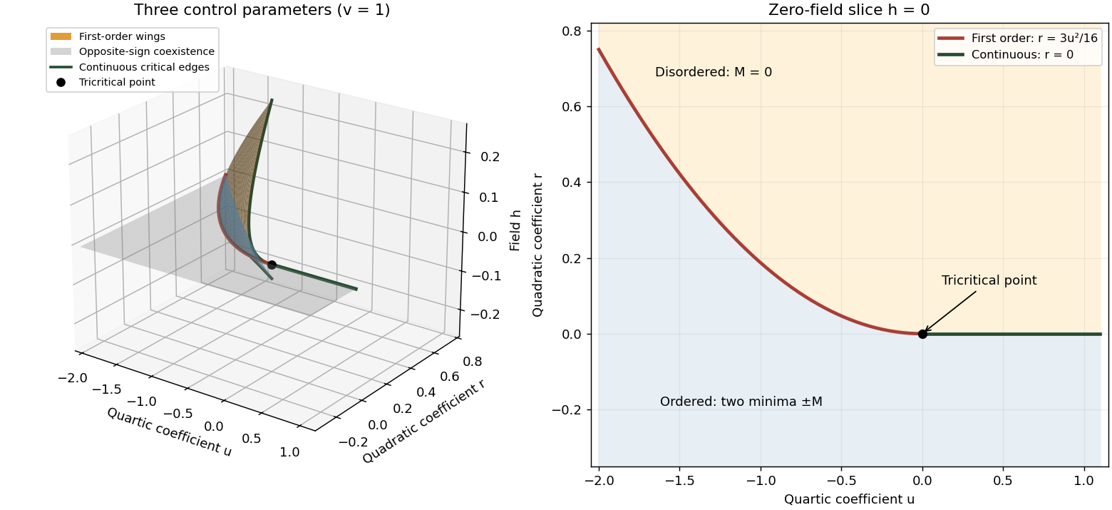
Tricritical phase diagram of the sextic scalar free energy: first-order sheets, critical edges and the zero-field slice
. Details. 
For the unheaded Ising model calculation, assume ferromagnetic exchange and let denote the mean Ising spin. On the hypercubic lattice the coordination number of a lattice is , even though the original positive-direction bond sum counts each bond only once. The mean-field approximation neglects products of deviations from :There are bonds, so the approximate energy is . Each independent Ising spin therefore sees the effective field . With , averaging its two Boltzmann weights gives the self-consistency equationThe slope of its right side at zero is , whereAbove , for excludes a nonzero solution. Below the initial slope exceeds one, and concavity of the hyperbolic tangent on the positive axis gives one positive solution and its negative partner. The Ising auxiliary mean-field free energy has positive quartic coefficient near , while its quadratic coefficient changes sign there. Its stable minima therefore move continuously away from zero; this is a continuous phase transition in the mean-field theory of the Ising model.
Put and . The Taylor expansion gives, on the nonzero branch,Consequently and the mean-field order-parameter exponent is . The inverse-temperature symbol used above is distinct from this order-parameter critical exponent.
For a ferromagnet the scalar order parameter is the spontaneous spin magnetization. It distinguishes a symmetry-invariant phase with zero mean from one of two phases with a nonzero mean of opposite signs. At zero field, a finite system with spin inversion symmetry has exactly zero mean. The spontaneous value is defined by taking the thermodynamic limit first and then sending the symmetry-breaking conjugate field to zero from one side.
A Landau-Ginzburg theory promotes the coarse magnetization to a scalar field and usesAt , spin inversion symmetry permits only even local powers. The gradient term penalizes spatial variations. The equilibrium statistical weight is ; the Landau approximation chooses a stable minimum of , whereas the full functional integral retains fluctuations around it. In a homogeneous phase this gives the equation of state . The field is conjugate to the order parameter, with .
Use the connected correlation function , since the disconnected constant in an ordered phase does not measure fluctuation decay. Away from criticality its large-distance exponential defines the correlation length:when that limit exists. Algebraic prefactors do not affect this definition.
Expand the Landau-Ginzburg theory about a stable homogeneous minimum . With , the quadratic fluctuation energy is . The Gaussian functional integral givesThis Ornstein--Zernike correlation function shows why the curvature of the free-energy minimum controls correlations. At a continuous phase transition that curvature vanishes, allowing long-range fluctuations. In the ordinary quartic theory with , above the transition and on either ordered branch below, so on both sides. At an equilibrium first-order transition the competing minima generally retain nonzero curvature, and the correlation length remains finite. The limit of local stability at a spinodal point is a distinct mean-field phenomenon.
Microscopically different systems can have the same critical exponents and appropriately normalized scaling functions. This universality means that they belong to one universality class when coarse-graining brings them to the same renormalization-group fixed point. Spatial dimension, order parameter symmetry and the range of the interactions affect that classification; changing a lattice spacing or a microscopic coupling generally changes nonuniversal amplitudes and the critical temperature instead.
In the scalar short-range Landau-Ginzburg theory, a positive quartic term and one thermal tuning produce ordinary Ising-type criticality. A generic sextic term does not change that fixed point, but tuning the quartic coefficient to zero exposes a different tricritical point with different exponents. The mean-field approximation itself neglects fluctuations. Its numerical exponents are reliable only when the Ginzburg criterion makes those fluctuations subleading; the ordinary scalar upper critical dimension is four, while the tricritical one is three. At an upper critical dimension logarithmic corrections can remain.
Set in the even sextic Landau free energy. For , near the nonzero stationary branch satisfies for . The minimum value is below the transition and zero above. The order parameter is continuous, and if crosses zero linearly with temperature, the first temperature derivative of the minimized free-energy density is continuous too. There is no latent heat; a second derivative has a finite jump at this level.
For , solve the two conditions and with . Setting gives and . Eliminating givesBoth the disordered and ordered minima have positive curvature there, but their values coincide. Crossing this phase coexistence boundary changes the global minimum discontinuously. The order parameter jumps; for at fixed , jumps as well, generically yielding a nonzero latent heat. Local extrema can persist past coexistence as metastable states, which explains hysteresis in a dynamically delayed transition. The spinodal points, where local curvature vanishes, do not locate the equilibrium transition.
The first-order coexistence curve approaches the continuous curve as : both meet at . To obtain this tricritical point, two even coefficients must be tuned to zero, while the sextic coefficient remains positive. A nonzero conjugate field removes the zero-field inversion symmetry and leads to the wing structure described in the root solution.
At , the equation of state becomes . For ,Above the transition and . These are stable branches of a bounded potential, and the ordered value tends continuously to zero at , but with rather than the ordinary square-root law. Tricritical behavior requires , and ; a generic path with fixed instead has ordinary critical behavior.
A critical exponent is the leading power of a singular observable as a control variable approaches a critical value. Use and distinguish the exponents from coefficient names in a Hamiltonian. Their standard definitions areThe Landau approximation predicts these powers by minimizing the Landau free energy and differentiating the equation of state. At an ordinary quartic point, , above and below, and on the critical isotherm. The equilibrium singular free energy is proportional to below, giving a heat-capacity jump. The quadratic fluctuation denominator is , so and . Thus the ordinary mean-field critical exponents areAt a tuned tricritical point, the preceding solution gives , and below. At the equation of state is . The curvature still vanishes linearly, and the Gaussian gradient term still gives zero anomalous dimension. ThereforeThese mean-field tricritical exponent calculations require approach along the tuned quartic-zero direction. Fluctuations modify the powers below the appropriate upper critical dimension, and marginal effects can add logarithms at it.
Take the connected correlation functionFor a massive phase its large-distance form is an algebraic prefactor times , defining the exponential correlation length . To specify the normalization of magnetic susceptibility, add to the energy and differentiate the mean spin. Translation invariance gives the correlation-function susceptibility sum ruleUsing the dimensionless source removes the prefactor . Below the transition, use a selected pure phase rather than a mixture of the two magnetizations, which would have a macroscopic disconnected fluctuation.
Choose a nonnegative blocking kernel normalized by . It may enforce a block average, a majority rule or a chosen rescaled coarse spin. Define the transformed weight bySumming this identity over coarse spins shows exact preservation of the partition function. The geometrical changes are and . A coordinate rescaling subsequently restores the reference cutoff if desired. The transformation is exact only if all generated operators are retained; a finite-coupling truncation is an approximation.
Define the coupling-independent term generated when byRestoring the original gives the identity-operator contribution to renormalization-group free energy:The parameter is an accumulated additive energy per coarse site. It multiplies the identity operator and leaves normalized spin probabilities unchanged, but it must be kept when calculating the absolute free energy. It records the eliminated-mode entropy and the normalization of their statistical measure.
Use an energy-per-site convention: and , so . Partition-function invariance givesConsequently, with ,This is the additive free-energy recursion under blocking. In a dimensionless free-energy convention multiply by ; the same recursion holds. The inhomogeneous term comes from the generated identity operator, not from a change in the spin-dependent couplings alone.
The affine equation naturally applies to the unsubtracted free energy. To extract its singular part, write and choose a regular background satisfying . Subtraction then gives . This analytic subtraction of an inhomogeneous renormalization recursion is justified when the eliminated finite-shell contribution is analytic near the fixed point and admits a regular subtraction. It can fail in a resonant direction, producing additive logarithms. The simple homogeneous formulas also assume the remaining irrelevant operators are not dangerously irrelevant couplings, and that marginal operators do not produce unaccounted logarithmic corrections. Calling the quantity in the affine equation “singular” does not make vanish automatically.
Near a renormalization-group fixed point , linearize the coupling map. In scaling coordinates , write to leading order. Here is a discrete multiplier, whereas is its logarithmic scaling exponent. A relevant operator has and grows under coarse-graining; an irrelevant operator has and decays. A marginal operator needs nonlinear analysis. Tuning the relevant fields to zero places the system on the critical surface. At the fixed point the spin field is rescaled as with . Its conjugate source therefore has . This accounts for both coupling and spin rescaling; the field normalization is part of the transformation, not a change in the physical microscopic spin length.
Assume the thermal field and magnetic field are the only remaining relevant directions. The homogeneous scaling hypothesis for critical phenomena givesChoose the stopping scale with . Thenwhere is the branch for and the branch for . Nonuniversal metric factors can be absorbed into the definitions of and these functions. Correlation lengths transform as , so . Differentiating the singular free energy twice with respect to temperature gives , and hence the hyperscaling relationTwo source derivatives similarly give . A single source derivative gives the ordered-branch exponent , and setting and scaling to one gives when the corresponding magnetization branch exists. These show explicitly how the critical exponents follow from the fixed-point scaling eigenvalues.
The independent correlation derivation uses with a single crossover scaling function. For lattice spacing , the singular continuum contribution to the magnetic susceptibility isHere is the area of the unit -sphere. The final integral is finite and nonzero when , is finite and nonzero, and the tail decays exponentially. Microscopic distances contribute a regular background. With this proves the Fisher scaling relationThere is an amplitude qualification in the printed large-distance formula: its tail has the Gaussian shape and, taken literally with amplitude independent of , integrates to a term proportional to . For a nonzero anomalous exponent it must instead be matched to the critical short-distance normalization. The matching the amplitude of a massive critical correlation tail givesAt this has precisely the same overall scaling as the critical form. Thus the requested identity uses the full scaling hypothesis, or equivalently this implicit amplitude factor. The printed tail without it is consistent as written in the Gaussian case .
Measure the statistical Hamiltonian in units of so that the weight is , and take , for convergence. Use the Fourier transform conventionThe last identity is the reality condition, so modes at and are not independent complex fields. Orthogonality of the Fourier exponentials gives , while a derivative multiplies a Fourier mode by . HenceThe kernel is positive for the stated parameters. Keeping an explicit inverse temperature instead would replace this kernel in the statistical weight by ; the following source convention absorbs that factor.
Couple a real source through . Its Fourier components obey , and the source term is . Complete the square using the positive quadratic kernel from the previous part:Translation of the integration variables in the regulated Gaussian functional integral therefore givesThis also fixes the sign: a real linear source increases the Gaussian generating function by a positive quadratic exponent, unlike an imaginary Fourier-characteristic-function source.
To specify rather than conceal an infinite normalization, first impose finite volume and an ultraviolet cutoff, and choose orthonormal real coordinates for the independent field modes. If their number is and the eigenvalues of the quadratic form are , the measure givesA measure removes the prefactor. In the continuum one may express this as plus a source-independent measure constant, with the same regulator understood. The real-mode prescription prevents double counting the conjugate Fourier pairs. All normalized correlation functions follow from and do not depend on that constant.
The connected generating functional is . Its second functional source derivative gives the connected correlation function; the source-independent determinant drops out. Translational invariance therefore givesThis covariance is independent of the source in a purely Gaussian theory; at zero source the mean field vanishes.
Fourier inversion can be evaluated with the Schwinger parameterization. Since , the elementary Fourier transform of a Gaussian giveswhere is the Modified Bessel function of the second kind. This integral formula also gives both asymptotic regimes directly.
For , set . The integral tends to the gamma function integral ; this is finite for . Hence, at distances larger than the microscopic cutoff,For , the exponent has its minimum at , with value . Gaussian expansion about that saddle, or the large-argument asymptotic expansion of a modified Bessel function, gives . ThereforeThis is the massive Gaussian field correlation tail with its normalization displayed. For example gives exactly , verifying both regimes and the exponential length scale.
Split the Fourier modes into and the shell . The source is uniform, so it couples only to the zero mode, which belongs to the retained part. The Gaussian field theory has no couplings between the shell and retained modes. Integrating out the shell therefore contributes only a source-independent determinant to the free energy, without changing the quadratic coefficients of the retained Hamiltonian.
Restore the cutoff by and choose the field normalization . Counting the measure, derivative and field factors explicitly givesThus in the convention that preserves the kinetic normalization, the Gaussian momentum-shell scaling isThe field has engineering dimension and zero anomalous dimension. The measure Jacobian and shell determinant supply the additive constant described in Q2. A different choice of field rescaling can redistribute factors into , but must give the same physical transformed correlation length .
At and the model is at a Gaussian fixed point. Its connected correlation function has the power-law critical form rather than a finite exponential decay length. Approaching from , the uniform susceptibility and the correlation length both diverge. If the thermal scaling field is linear in with finite and positive, thenThe same result follows from the mass multiplier : its logarithmic thermal eigenvalue is two, so .
The determinant also shows a thermodynamic singularity. Two derivatives of the free-energy density with respect to give, up to sign and a nonzero normalization,as . Rescaling establishes the power, and the dimensionless integral is ultraviolet-convergent for . Integrating back gives a nonanalytic free-energy term proportional to after regular backgrounds are removed. This is critical behavior of the quadratic model.
There is a stability qualification: a pure Gaussian potential with is unbounded below in the uniform mode, so it does not by itself provide a stable ordered phase on the other side. The ordered-phase obstruction in a Gaussian scalar model is removed by adding a positive quartic interaction. In that interaction is relevant, so the resulting generic scalar critical point need not retain the Gaussian exponents. Thus the calculation proves the Gaussian critical singularity and , without claiming that the unmodified quadratic integral defines both phases of a physical ordered transition.
Assume short-range ferromagnetic exchange and zero external field. In the one-dimensional Ising model, a domain wall costs only , independent of the lengths of the domains it separates. There are order- positions for one wall, so its positional entropy offsets any finite energy cost at nonzero temperature as the system grows. Domain walls consequently have a positive density at every , destroying a uniform spontaneous spin magnetization. Periodic boundaries require an even number of walls, but that constraint does not remove their nonzero thermodynamic-limit density.
The One-dimensional Ising correlation function makes this argument explicit. A bond is broken with probability , and the infinite-chain correlation isThe dominant eigenvalue of the transfer matrix for the one-dimensional Ising model is , so the free energy per spin is analytic for . There is no finite-temperature transition in one dimension; only the zero-temperature limit orders.
In two dimensions a reversed cluster is enclosed by a Peierls contour. A contour of length costs , while the number of such contours surrounding a fixed site grows at most as a polynomial in times : after the initial edge, a nonbacktracking square-lattice walk has at most three choices per step. With plus boundary conditions, flipping the interior of a specified contour yields the Boltzmann suppression . ThereforeFor sufficiently low temperature this bound is below , giving a positive spontaneous magnetization. This is the energy-entropy mechanism of the Peierls argument.
At sufficiently high temperature, the graphical expansion bounds correlations by sums of connecting paths weighted by . The same nonbacktracking count converges geometrically when , giving exponential decay and a disordered phase. Since an ordered low-temperature phase and a disordered high-temperature phase both occur, the two-dimensional model has a finite-temperature phase transition. The argument establishes its existence and the dimensional distinction, not the exact value of its critical temperature.
Write and take . The unit-length constraint prevents an arbitrary multiplicative field rescaling, so the running coupling is found by renormalizing the coefficient of . We compute that coefficient in a slowly rotating planar background, which is enough because symmetry makes the two-derivative stiffness isotropic on the sphere.
Let , and for the remaining constant orthonormal tangent vectors. Parameterize the fast tangent fluctuations byThis satisfies exactly. Put , and choose it locally constant and small compared with the shell momenta. Since and , direct differentiation givesAt quadratic order in the fast fields, the cross term is , whose integral is zero for constant . The term is quartic in the fast fields. Remaining cross terms are cubic and have zero Gaussian expectation; their effects on the two-derivative stiffness start at higher loop order. Field-measure corrections independent of the background contribute normalization terms and do not alter the leading gradient coefficient in this calculation.
The quadratic fast action is . In the shell its connected correlation function is with the momentum delta function understood. Thus , wherewith the limit . Here is the angular measure of the unit -sphere. Averaging the background-gradient coefficient gives the one-loop stiffness of a spherical nonlinear sigma model:The coefficient is , not : the fluctuation tangent to the rotation plane does not reduce the gradient cost, because its contribution cancels between and . All other transverse components do reduce it.
After integrating out the shell, put to restore the cutoff. The constrained field keeps unit norm, so , or at this orderFor , . Therefore the renormalization-group beta function isThe displayed terms are the requested one-loop flow. They are a weak-coupling expansion; the discrete target has no tangent modes and must instead be treated by domain walls, as in the first part.
Set . The one-loop flow is . For and , its physical fixed points areThe zero point attracts small positive couplings, whereas the nonzero point is the separatrix between the low-temperature weak-coupling flow and the strong-coupling regime. This is a perturbative description for small ; extrapolation of its nonzero root to large is not controlled.
At and , the only finite one-loop fixed point is , a double root. Positive flows to strong coupling. For the loop coefficient vanishes: at only is fixed, while at every is fixed in this perturbative spin-wave description. The compact two-component model also admits vortices; their Berezinskii–Kosterlitz–Thouless transition is absent from a calculation retaining only the smooth tangent modes. Thus a zero beta function here does not exclude that transition. The formula should not be interpreted as a continuum result for the discrete Ising target.
For a fixed point , put . Linearizing the renormalization-group flow givesBecause is proportional to temperature at fixed microscopic stiffness, this derivative is the thermal eigenvalue. The thermal eigenvalues of the spherical nonlinear sigma model areThe first value describes the stable zero-temperature ordered fixed point. At the nonzero critical point the thermal perturbation grows as , so the stopping scale gives and to leading order in the expansion. Higher-loop terms change this to .
At the linear eigenvalue is zero, so its sign alone does not decide the flow. For the first nonlinear term is positive. Integrating it givesThe flow reaches order-one coupling at a length logarithm of order , explaining the exponentially large correlation length in a two-dimensional spherical sigma model rather than a finite-temperature power-law critical point in this smooth-field regime. For , , the linear eigenvalue is zero everywhere on the perturbative line and vortex effects require an additional coupling. For , , the sole zero-coupling fixed point has .
Articles by others on the same topic
There are currently no matching articles.