The target specifies the desired output; the controller selects a control input; an actuator realizes it on the system; and the sensor returns a measured output. The environment supplies additional interactions and disturbances. A simple loop is:
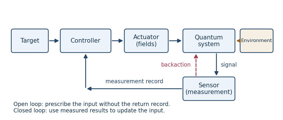
Quantum control loop, showing the measurement record and measurement backaction
. Details. 
For a quantum sensor, a measurement in quantum mechanics has statistical outcomes and generally changes the state through measurement backaction. For example, outcome of an instrument with operator has probability and conditional stateA single unknown quantum state cannot generally supply its complete instantaneous state vector to a controller. Noncommuting observables cannot be read simultaneously with arbitrary precision, and reliable quantum state tomography normally needs many reproducible preparations. A conditional state estimate can instead be updated from a continuous record, with its disturbance included in the model.
Quantum actuators change a Quantum Hamiltonian through applied electromagnetic fields, tunable interactions or couplings to auxiliary systems. A closed-system actuator implements unitary operators, so it preserves the spectrum and purity of a density operator; it cannot arbitrarily overwrite a state as a classical assignment operation could. Dissipative actuators or measurement in quantum measurements can change these invariants, but their dynamics must be accounted for.
The environment can entangle with the system, causing decoherence and dissipation when unobserved degrees of freedom are traced out. It is consequently part of the dynamical model, rather than just an additive classical disturbance. Conversely, Markovian reservoir engineering uses such coupling constructively to prepare and stabilize states.
In open-loop control the applied waveform is prescribed without using measurements from the current evolution. In closed-loop control it depends on the available measurement record or inferred state. Measurement-based quantum feedback is one realization of the latter; experimental adaptation across repeated preparations is another. The measurement record is classical information, but its production has quantum backaction.
Three standard objectives are state preparation, observable optimization and process implementation. All optimizations are over admissible control inputs and a specified final time .
For state preparation, steer an initial density operator to a target . An exact goal is , or one may minimize the squared Hilbert-Schmidt distanceFor a pure target , maximizing is a useful alternative. The target must be physically attainable: Hamiltonian engineering alone preserves the initial spectrum of the density operator.
For an observable objective, choose a Hermitian operator and maximize its expected final value:Population transfer is a special case with the projector onto the desired level or subspace; suppressing an unwanted population reverses the sign or minimizes this quantity.
For coherent process engineering, implement a target unitary operator on every input, rather than merely arranging one state transfer. If the propagator is , a phase-insensitive error isThe error vanishes precisely when : equality in the Hilbert-Schmidt inner product Cauchy-Schwarz inequality bound makes the two operators proportional. For an open-system process, the analogous objective compares the implemented quantum channel with the target channel. These objectives can be supplemented by pulse-energy, amplitude, bandwidth and duration constraints in quantum optimal control.
A reachable set consists of states obtainable from one specified initial state using admissible inputs and allowed durations. Controllability means that every target in the declared state space is reachable from every initial state there; the declared space and time convention are essential.
For a closed quantum system, let solve the controlled Schrödinger equation with . The propagator and state reachable sets areA pure-state version acts on normalized vectors up to global phase. Pure-state controllability makes every pure target accessible; unitary operator controllability permits every desired coherent process, with global phase treated according to the definition.
For mixed states, density operator controllability means transitivity on each unitary orbit of a density operator, not access to all density operators regardless of spectrum. The Dynamical Lie algebra generated by describes the accessible connected unitary transformations under the usual unconstrained-time control assumptions. Conserved quantities or restricted controls can shrink the reachable set. Thus successful preparation of one state is weaker than implementation of an arbitrary gate on all inputs, and coherent controllability does not imply purification.
Hamiltonian engineering chooses accessible interactions so that their actual or effective Quantum Hamiltonian produces the desired evolution. A typical model is ; the controls may change frequencies, amplitudes, phases or coupling strengths. Three standard model-based open-loop control approaches illustrate different mechanisms.
In resonant quantum control, select a transition with a near-resonant field. In a rotating frame, after neglecting rapidly oscillating terms in a justified regime, an effective two-level drive can be . When its axis is fixed,The pulse area sets the rotation angle and the drive phase selects the transverse axis. A resonant pulse of area swaps the two level populations. This requires knowledge of transition frequencies, couplings and the validity of the selective-drive approximation.
In adiabatic quantum control, design a slowly varying Quantum Hamiltonian whose desired instantaneous eigenstate connects the initial and final states. For a nondegenerate eigenstate separated by a gap, the quantum adiabatic theorem explains why sufficiently slow evolution follows that state up to a phase. The relative size of matrix elements of and squared spectral gaps controls the approximation; degeneracies or rapid changes invalidate simple following. This engineers a state path rather than a prescribed resonant rotation.
In average Hamiltonian engineering, apply a predetermined sequence of fast pulses and let the system evolve for intervals in the corresponding frames. For cycle length , the leading effective generator isChoose the sequence to cancel unwanted terms or retain desired couplings. For instance, equal intervals under and its conjugate cancel the leading generator because . Noncommuting terms produce higher-order commutator corrections, so fast cycling, finite pulse errors and the accuracy of the model matter. All three methods determine a waveform or sequence before its execution; none automatically corrects an unknown mismatch during that run.
Replace evaluation in a possibly inaccurate dynamical model by an experimental objective. Parametrize an admissible pulse as , with collecting time-slice amplitudes or basis-function coefficients. Prepare the same initial state, apply the pulse, measure performance, and update before the next run. This is adaptive experimental quantum control: the loop closes through experimental results, even though each individual pulse is applied open loop.
For example, minimizefor a pure target , with a nonempty closed convex set enforcing amplitude and bandwidth bounds. The overlap is an experimentally estimable probability. An observable objective can use its measured expectation instead; a gate objective generally needs more input states and measurement settings. The true dynamics constrain the physically produced , but no accurate formula for those dynamics is required to evaluate this objective.
A direct search compares measured scores for candidate pulses, accepts improvements and refines the search region. Alternatively estimate a gradient experimentally by finite differences,where is the Euclidean projection onto a convex set. Population-based searches can also explore several candidates in parallel. These methods use experimental data rather than simulated propagation or a model-derived adjoint gradient.
Each score needs enough repeated preparations to manage measurement noise; uncertainty in score differences should determine replication and stopping decisions. Excessively small finite-difference steps amplify that noise. A model-based pulse can provide a useful starting point, but adaptation corrects its systematic mismatch using the device itself. This mitigates model uncertainty, not arbitrary fluctuations: reproducible preparation, calibrated measurements and sufficiently slow drift remain necessary. Nor does a local numerical search guarantee a global optimum.
Articles by others on the same topic
There are currently no matching articles.