For a bounded linear operator between Hilbert spaces, the Moore–Penrose inverse of an operator assigns to each admissible datum its unique minimum-norm least-squares solution. Its domain isWrite , where and . Then . Restricting to removes the ambiguity among solutions differing by an element of the kernel. The orthogonal decomposition also shows that is the orthogonal projection of onto , and is the orthogonal projection of onto . The inverse is defined on a dense domain and need not be a bounded linear operator when the range is not closed.
The given map is the unilateral shift operator. Its adjoint operator is the left shift operator, sinceThe shift is an isometry with trivial kernel and closed range . Its range has orthogonal complement , so every square-summable datum is admissible. Consequently,Indeed , while is the required orthogonal projection. The discarded first component is the residual of the least-squares solution, not an obstruction to the existence of the Moore–Penrose inverse of an operator.
Choose a singular system of a compact operator with , and . The Picard criterion, together with range orthogonality, givesFor necessity, expand a solution's component in in the orthonormal vectors ; its coefficients must be . Their square sum is finite by Bessel's inequality. Conversely, the displayed square sum defines a convergent Hilbert space seriesApplying the bounded linear operator to the partial sums yields the expansion of in . Thus its limit solves . The perpendicularity condition is essential here: the Picard criterion alone characterizes the domain of the generalized inverse, which also includes components in .
A linear regularization is a family of bounded linear operators , , for which for every as . To obtain a convergent regularization of an inverse problem for noisy data, choose a regularization parameter so that the exact-data approximation error and the amplified noise both vanish.
An example is Tikhonov regularization:The positive quadratic term makes invertible. The Tikhonov filter norm bound follows from the filter , whose maximum for is . Therefore . The spectral factors tend to one on the positive spectrum; dominated convergence theorem gives consistency on . The noise-bias decomposition for linear regularization then proves convergence whenever and , for example for sufficiently small positive noise levels.
The Volterra integration operator is injective and has dense range. Its range of the Volterra integration operator is , and its Moore–Penrose inverse of an operator is differentiation on this domain. Thus the error estimate for implicitly requires , in addition to the printed assumption. For an arbitrary function the same calculation bounds error against , but that function need not be in .
Put , and . The three stencils are forward, central finite differences, and backward on , and , respectively. All shifted evaluation points lie in . For , apply and change variables in each of the six evaluation terms. The resulting integration intervals arePair with , with , and the two middle intervals. Each pair has disjoint interiors, so almost every point is counted at most three times. This overlap multiplicity bound for piecewise difference operators provesFor the bias on the middle interval, write the central finite difference as an average of . The fundamental theorem of calculus giveswhere . Extend by zero to the real line. Young's convolution inequality bounds the middle-interval error by . Combining its squared error with the supplied outer-interval estimate gives the central-difference noise-bias boundThe triangle inequality and the operator norm estimate now giveFor , balancing noise and approximation bias minimizes this upper bound atfor sufficiently small that . Capping the parameter at supplies an admissible rule for all positive noise levels. More generally, and suffice; avoids needing or dividing by .
To prove convergence for every admissible datum, not just data, let with and extend by zero. Each stencil is a forward, centred or backward average of . Translation continuity in Lp makes each averaged difference from tend to zero in . Restricting those three bounds to their respective intervals proves . The noise-bias decomposition for linear regularization, with , finishes the convergent regularization of an inverse problem.
For a proper convex function on a real Hilbert space, its subdifferential at isIn a Banach space, interpret the pairing with an element of the dual space. For a chosen subgradient , the Bregman distance isIf also , its symmetric Bregman distance isThe subgradient inequality proves nonnegativity. These quantities depend on the chosen subgradients and generally are not metrics: they need not distinguish different points or obey the triangle inequality.
For the maximum-entropy regularization functional, differentiation of the scalar integrand gives . Thus the Fréchet derivative at a positive reference function is , and the stated differentiability result gives . Consequently,This is the generalized Kullback–Leibler divergence. When both functions integrate to the same mass, the last two terms cancel after integration; for probability density functions it becomes the usual Kullback-Leibler divergence. For two positive functions, adding the reverse distance givesA sufficient setting for the differentiability argument is with bounded away from zero. For nonnegative , use wherever appropriate. Positivity alone in does not automatically provide an open domain on which the Fréchet derivative exists.
For , the subdifferential at zero is . Choose the allowed interior subgradient . Its supporting line is horizontal, so the Bregman distance is the vertical gap from to at the selected input:More generally, an interior choice gives . The sketch shows the particular choice .
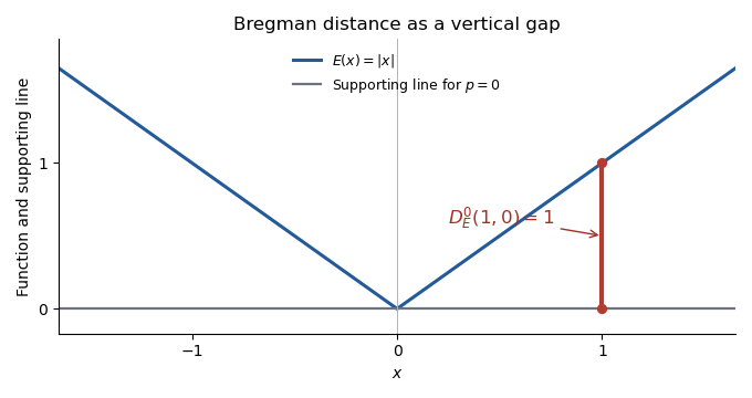
Bregman distance for the absolute-value function at x=1 from the reference point zero, using the subgradient p=0
. Details. 
Interpret the normal-operator source condition as the displayed intersection condition: there is with . Fix any and put . The subgradient optimality condition for the artificial-data objective isIt holds because its first term equals . By convexity, this is sufficient for global minimality, proving the forward implication. Conversely, if minimizes that objective, the same optimality condition givesTaking proves the intersection condition. Thus the two conditions are equivalent when the source vector is allowed to be zero.
The printed additional requirement is not equivalent in general. For and , the displayed source condition holds, and choosing makes the minimizer, but forces . A nonzero-source version needs an additional hypothesis, such as requiring ; it cannot be inferred from the printed intersection alone.
Let from the normal-operator source condition, and set . Since is a least-squares solution, the normal equation for a linear inverse problem gives . Expand the objective difference and use the Bregman distance definition:The cross term with the residual of the least-squares solution vanishes by the normal equation; exact data are not required. Compare the minimizing with . At , the completed square is zero. Dividing the resulting inequality by proves the stronger shifted-comparator Bregman boundDropping the nonnegative squared term gives the requested estimate. If the comparator lies outside the effective domain of , its distance is infinite and the inequality is valid but gives no finite error bound.
The relevant nonlinear generalized singular vector relation, without imposing unit-data normalization, isThis is a generalized eigenfunction in the forward-operator metric, rather than a distributional generalized eigenfunction of a linear operator. It supplies the normal-operator source condition with . For a convex positively one-homogeneous functional, the subgradient inequality applied at zero and at gives . If , thenAssume the usual positive eigenvalue and . By positive homogeneity,The shifted-comparator Bregman bound therefore yieldsThe vector is itself a minimizer: remains a subgradient along the nonnegative ray, and substitution satisfies the subgradient optimality condition. If is injective, this also proves . Otherwise distinct minimizers can differ in the kernel while sharing the same predicted data.
For a nonnegative convex positively one-homogeneous functional, the branch continues as above the threshold, since there. Nonnegativity is needed for that clipping argument; bare positive homogeneity allows signed linear functionals.
Zero Bregman distance does not imply exact recovery. For , , and , the minimizer is , but . Both points touch the same supporting line, as described by zero Bregman distance and supporting faces.
For a proper convex function that is lower semicontinuous on a Hilbert space, its proximal operator at scale isThe minimizer is unique because the objective is strongly convex; existence follows from the closed proper convex functional and the coercive quadratic, using an affine lower bound. The subgradient optimality condition is , which is exactly the displayed resolvent of a monotone operator relation. Setting gives the unscaled proximity or resolvent operator requested here. This is a nonlinear resolvent of the subdifferential, distinct from the spectral resolvent of a linear operator.
Let and assume . The scalar Poisson data fidelity integrand has derivative . Applying the permitted interchange of differentiation and integration in a direction givesThus the ambient-space Fréchet derivative, or its Hilbert space gradient when the pairing is an inner product, isThe quotient is pointwise, and the adjoint operator transports it back from the data domain to the source domain. The chosen spaces must ensure the integrals and derivative pairing are finite; an output bounded away from zero is a useful sufficient condition.
The printed set of probability density functions and positive cone are not vector spaces, so the notation for a bounded linear map between them is understood as a positive bounded linear operator on ambient function spaces, restricted to admissible inputs. If unit mass is a constraint, admissible directions satisfy . The displayed gradient is then a representative modulo an additive constant; optimization with that constraint additionally includes its normal cone.
For the quadratic case, write and . Since is an orthogonal matrix, the quadratic proximal term becomes . The subgradient optimality condition givesAll , so each diagonal entry is positive, including when . Multiplying by the inverse diagonal matrix givesThe proximal operator of Poisson data fidelity separates pointwise. At each , the scalar optimality equation on isSince , the two roots have opposite signs. Only the positive root is admissible in the logarithm:The negative root is outside the effective domain. The second derivative of the proximal objective is positive, establishing the unique pointwise minimizer. The integral formula is understood on the function spaces where these quantities are admissible.
Finally, for , positive and negative minimizers obey and , respectively. At zero the subdifferential condition is . Combining these cases yields soft thresholding:Thus supplies all three requested closed forms.
For the convex conjugate, use a dual scalar to avoid confusing it with the fixed centre . Differentiating gives , so the unique maximizing point is . Substitution yieldsThe positivity of makes the maximized quadratic strictly concave and the convex conjugate finite for every real .
Take with the usual proper closed convex assumptions, so the Fenchel-Moreau theorem identifies its conjugate with the supplied . Put . The first update is . By Moreau decomposition, the second update isAlso , so the argument in the final update contains . Eliminating the auxiliary variable givesThis is the primal-dual hybrid gradient method with extrapolation parameter one and the primal update performed first. Its saddle point function is , corresponding to the primal objective .
For proper lower semicontinuous convex functions and a nonempty saddle-point set in these finite-dimensional spaces, the standard convergence of primal-dual hybrid gradient theorem gives the sufficient parameter conditionHere is the operator norm, or largest singular value. For , one possible choice is with ; for any positive steps satisfy the condition. The existence assumption is necessary: step sizes alone cannot guarantee convergence to a saddle point that does not exist.
Articles by others on the same topic
There are currently no matching articles.