Past exam of the MPhil in micro- and nanotechnology enterprise course of the University of Cambridge / 2020 / Paper 1 / Section A(i)

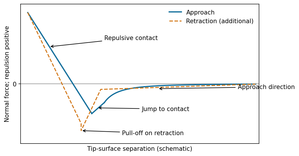
The atomic force microscope measures the cantilever deflection $d$, converted to normal force by $F=k_{c}d$ after calibration. On approach, the force is initially almost zero, then attractive; a sufficiently steep attractive force gradient causes jump-to-contact. After contact, further approach bends the cantilever and indents the sample, giving a rising repulsive branch. With tip-surface separation increasing to the right, approach proceeds from right to left. The instability occurs when the magnitude of the attractive force gradient exceeds the cantilever stiffness. The contact-branch slope depends on both cantilever and sample compliance.

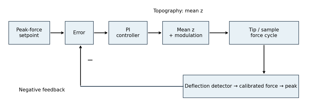
The controlled quantity is the maximum repulsive force in each tapping cycle. In PeakForce quantitative nanomechanical mapping, a vertical modulation below the cantilever resonance produces a force-distance cycle at each pixel. The optical lever measures deflection; the calibrated cantilever stiffness converts this to force. Subtract the measured peak force from the setpoint and use proportional-integral control to adjust the mean vertical scanner position. Excessive peak force makes the controller withdraw the sample or tip; insufficient force makes it approach. The scanner position required to maintain the setpoint supplies the topography signal. This controls the top of the repulsive branch in the preceding curve, rather than the oscillation amplitude used in conventional tapping mode.^[ref]

Two useful properties are adhesion and contact elastic modulus. The pull-off force, the most negative force on retraction relative to the noncontact baseline, maps adhesion. Fit the contact part of the force-indentation relation using a suitable contact mechanics model to obtain a reduced elastic modulus; for example, the DMT contact model useswhere $F_{\mathrm{adh}}<0$, $R$ is the calibrated tip radius and $\delta$ is indentation. Converting $E^{\ast }$ to a sample Young's modulus also requires the tip modulus and the two Poisson's ratios. The approach curve alone does not supply a retraction pull-off measurement. The loop area can additionally map dissipated energy; it is not automatically a purely viscous loss.^[ref]

Treat the magnetic electron lens as a paraxial thin lens. A point in the specimen sends rays through different lens positions; the lens brings these to a conjugate point in the image plane, with $1/u+1/v=1/f$ and transverse magnification $-v/u$. Conversely, waves leaving different specimen points at the same angle are focused to the same point in the back focal plane. This plane therefore contains the electron diffraction pattern, with radius $r\simeq f\theta$ for small scattering angle $\theta$. The specimen is just beyond the front focal plane, giving a magnified real image farther downstream.

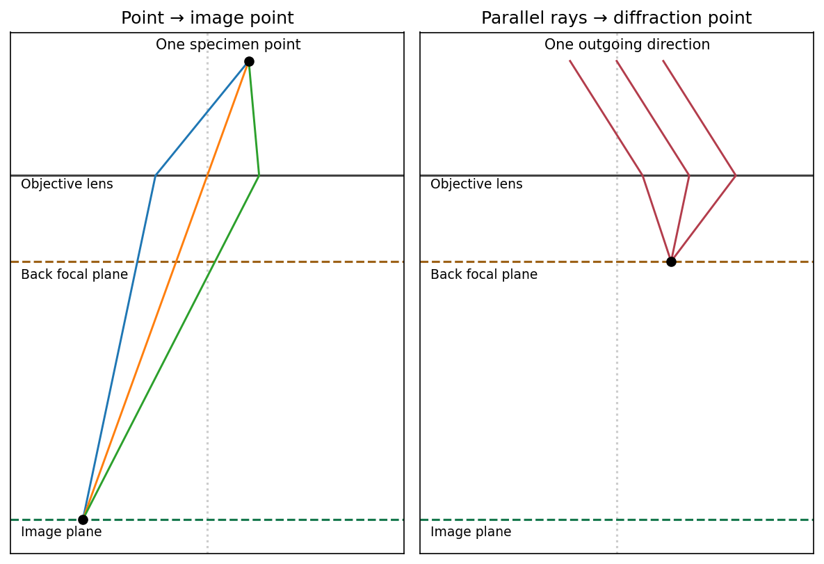
The sketch assumes a thin specimen, coherent approximately parallel illumination, small angles and an ideal lens without aberrations. Quantitative diffraction intensities may require dynamical scattering; the ray sketch only establishes the plane conjugacies.^[ref]

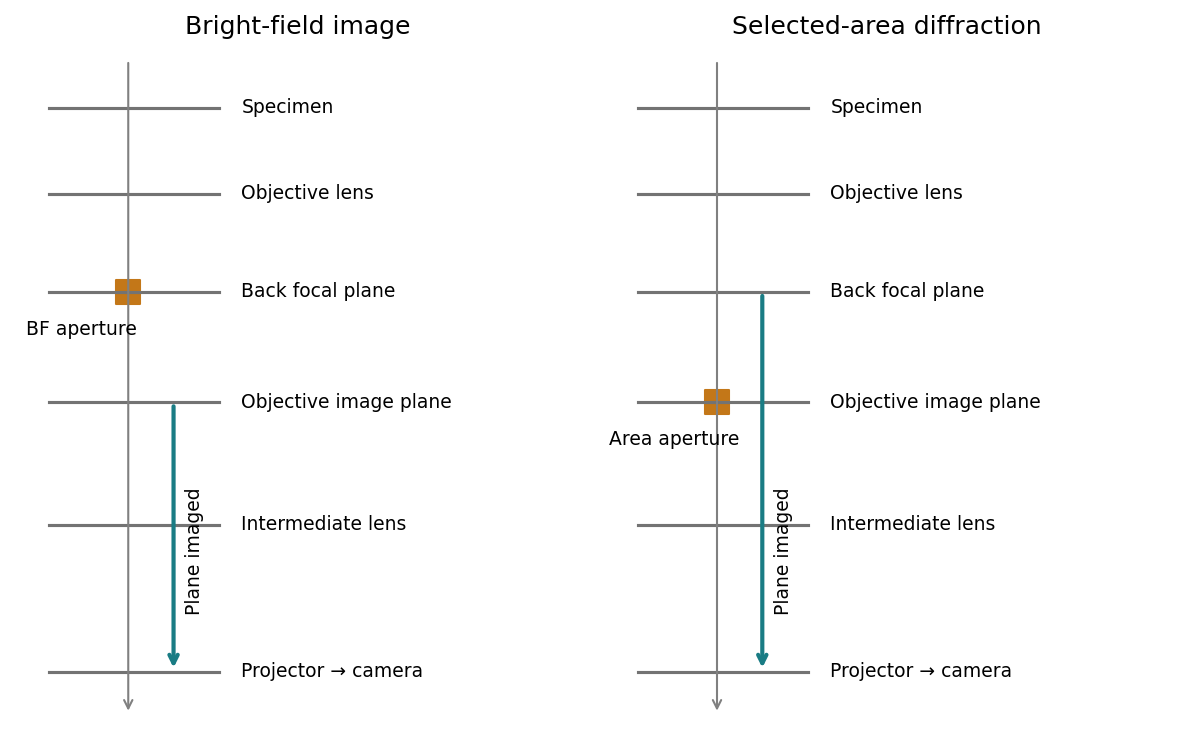
For bright-field transmission electron microscopy, place the objective aperture in the back focal plane around the transmitted beam, excluding most diffracted beams. Adjust the intermediate lens to image the objective's real-space image plane; projector lenses enlarge that image onto the screen or camera. Regions removing electrons from the admitted beam tend to be darker, although phase contrast can also contribute.

For selected-area electron diffraction, put the selected-area aperture in the objective image plane to choose a specimen region. Remove or open the objective aperture and change the intermediate-lens excitation to image the objective's back focal plane onto the camera. The projector then magnifies the diffraction pattern, rather than the specimen image. Thus the two apertures act in different conjugate planes.

The resolved graphitic fringes indicate high-resolution phase contrast in a multi-walled carbon nanotube. Interference of transmitted and diffracted electron waves produces lattice fringes; their darkness is controlled by defocus, thickness and the contrast transfer function, so a dark fringe is not an unqualified map of individual carbon atoms. The weakly scattering central channel is lighter than the multilayer walls. Curved, roughly parallel fringes at its sides identify concentric graphitic shells; the dense fringes at the lower edge arise from overlapping graphitic material or another tube, not necessarily the wall count of the central tube.

Using the printed $5\mathrm{nm}$ scale bar, the central tube has an outer diameter of roughly $9$–$10\mathrm{nm}$ and an inner channel of roughly $6$–$7\mathrm{nm}$, depending on the cross-section selected away from the overlap. Several wall fringes are resolved on each side, with separations of order $0.34\mathrm{nm}$, consistent with graphitic interlayer spacing. These are approximate image measurements, not a determination of chirality, chemical purity or an exact shell count. The image alone cannot establish those quantities.