Use Gaussian elimination with partial pivoting, choosing a largest absolute entry in the uneliminated part of each pivot column. The first pivot is two in row one, with multipliers for rows two, three and four. The second-column candidates are then , so row two stays as pivot and the remaining nonzero multiplier is for row four. The augmented matrix at this stage isThe third pivot is three, so swap rows three and four. The final multiplier is , leaving last pivot . Carrying that swap through the previously stored multipliers givesThe transformed right side is . Back substitution gives , , and , hence .
For the eigenvalue claim, put . It is invertible because a permutation matrix and a unit lower triangular matrix are invertible. The factorization gives , soSimilar matrices have the same characteristic polynomial and therefore the same eigenvalues with algebraic multiplicities. This proves the claim without changing the prescribed elimination method.
A natural cubic spline is piecewise cubic, interpolates the data, has continuous first and second derivatives at the knot, and has zero second derivative at the outer endpoints. Its nodal second derivatives here satisfy and the usual matching equationso . The resulting pieces areDirectly, the values are , both first derivatives at one equal two, both second derivatives there equal six, and . Thus all spline conditions hold.
The second data set adds the values of the affine function to the first. Adding to the spline preserves derivative matching and the zero endpoint second derivatives, so uniqueness of the natural interpolant gives the new spline . Its first piece is , and its second is . This is the affine covariance of natural cubic spline interpolation.
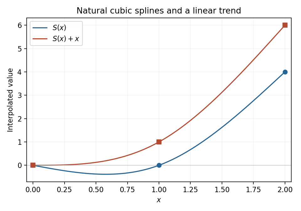
Natural cubic interpolation and an affine change of the data
. The second interpolant is obtained by adding to the first. Dots mark the three interpolation nodes of each curve. Details.
Articles by others on the same topic
There are currently no matching articles.