Write the complex potential of a two-dimensional potential flow as , and the complex velocity as . The lower solid wall has . The upper solid wall and its continuing free streamline have constant equal to the far-field volume flux per unit depth, namely . Consequently the potential domain is the infinite stripThe points correspond to , to , and is by the chosen potential normalization.
In the hodograph plane, the horizontal wall has real positive, the vertical wall has imaginary positive because the physical velocity is downward, and the fluid free boundary has . The upstream reservoir velocity tends to zero, the outgoing velocity is one, and the velocity at is . Thus the hodograph is the first-quadrant unit quarter disk, with at , at , and at .
For the potential strip, exponentiation followed by a Möbius transformation givesSince lies in the upper half-plane, so does . The map sends to , to infinity, and to zero.
For the first-quadrant hodograph plane, successively square , apply , and then use a negative square:The first map takes the quarter disk into the upper half of the unit disk. The fractional transformation takes this to the second quadrant, whose negative square is the upper half-plane. The boundary points map to , as required. Uniqueness of the normalized conformal map therefore identifies the two expressions:
On the free streamline choose with . The lower endpoint of this parameter interval is , and approaches . The fractional expression in the map isHence , and the branch on the upper edge of the potential strip isDifferentiate to obtain . Since , the chain rule givesThe sign and interval are consistent with the free surface moving to the right and downward from .
Separate the real and imaginary parts of the derivative and integrate from :Because and , these integrals areAs , and . This must equal the outgoing stream depth , so
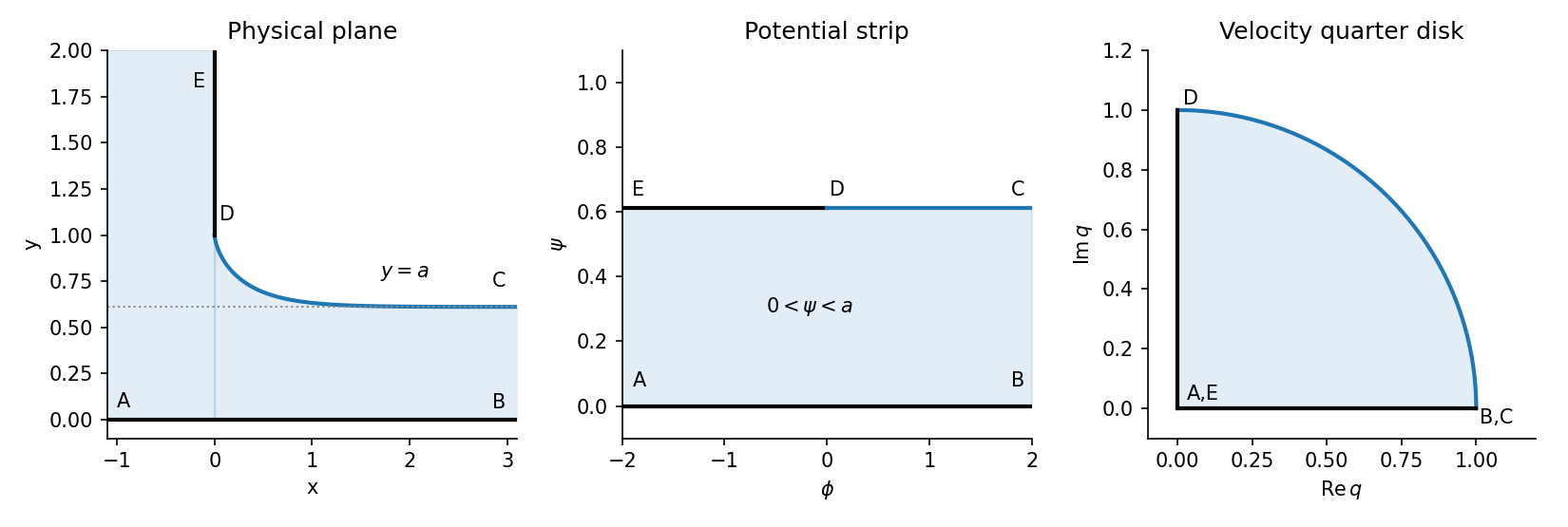
Draining free surface and its potential-strip and hodograph representations
. Details. 
The solution has a vertical tangent at and approaches the horizontal line downstream, agreeing with both solid-wall and free-streamline conditions.
Orient the contour so that the plus side is on the left; for a positively oriented simple closed contour this is its interior. If is a smooth arclength parametrization with , define the Cauchy principal value by deleting a symmetric interval and taking . This pairs the two singular sides at equal local arclength.
Near , write . The second term divided by is regular because is analytic there. For the constant term, indent the contour on either side of by a small semicircle. Its limiting contribution to the Cauchy integral is , while the remaining contour tends to its principal value. This proves the Sokhotski–Plemelj theorem:In particular and for the given integral equation.
Define inside and outside. Its jump is , and it vanishes at infinity. ThereforeIndeed, the difference between the two sides has no jump, extends analytically across the smooth contour, and vanishes at infinity; Liouville's theorem makes it zero. Applying the Sokhotski–Plemelj theorem again,Thus the normalized closed-contour singular integral operator is its own inverse.
For an admissible Laplace integral solution, differentiation under the integral sign and integration by parts giveChoose endpoints for which the boundary term vanishes. Setting the density in braces to zero givesTwo suitable contours are the rays and , with a continuous square-root branch on each ray. The Gaussian decays at infinity, and tends to zero at the finite endpoint. The integrals converge for every finite .
To check independence rather than merely exhibit different paths, defineWith unit normalization, the two solutions satisfy and . Their Wronskian at zero is , so they form an independent pair.
Strictly, the printed necessity claim requires an injective contour-transform class as well as vanishing endpoint terms. An arbitrary contour representation may contain a null weight in a contour Laplace representation, so a nonzero solution alone does not force every representing to have the displayed form. The calculation constructs the canonical density and two valid independent solutions; it does not assume uniqueness for unrestricted contour densities.
Extend to be zero for . Define for andThen the full-line equation is . Use the Fourier transform conventionUnder the corresponding growth bounds, the positive-support transform is analytic above a horizontal line and the negative-support transform below a horizontal line. If both functions have suitable subexponential growth, the basic domains are respectively the upper and lower half-planes; exponential decay can enlarge these to overlapping strips. The convolution theorem gives .
The Wiener-Hopf method factors into functions analytic and nonzero in the respective domains. After multiplicative or additive separation, the two sides continue to one entire function, whose growth determines a polynomial by Liouville's theorem. Real-axis zeros must be assigned consistently with the inversion contour, rather than divided out without specifying a side.
For , direct integration gives , soRearrange the Wiener-Hopf factorization asThe left side has the positive-support analytic continuation and the right side the negative-support one. Their growth, from the supplied bounds, makes the common continued function a constant . ConsequentlyFor this kernel, on the negative axis is a multiple of , so the latter transform is analytic for . The common strip can therefore be chosen as . In particular the inversion line must pass above both real poles of .
Set . ThenThis is the transform, on , ofEquivalently, Fourier inversion closed below the inversion line for picks up the two real poles with clockwise orientation.
As a direct check, let . Since , the equation gives . At zero, differentiation of the integral gives , so ; this sets the sine and cosine coefficients equal. Direct substitution, or the transforms above, then verifies the full integral equation, not merely its differentiated form.
Articles by others on the same topic
There are currently no matching articles.