Past exam of the physics A course of the University of Cambridge / 2015 / Paper 1 / Section A

The Born rule uses the squared modulus, so the imaginary term contributes positively: $|a+ix{|}^2=a^2+x^2$. For $a>0$, wavefunction normalization would multiply the supplied expression by $N=\sqrt{3/(4a^3)}$. Equivalently, take the ratio of the integrals directly:Using ${\psi }^2$ instead of $|\psi {|}^2$ would fail to produce a real, nonnegative probability density.

For the quantum harmonic oscillator, put ${\ell }_0=\sqrt{\hslash /(m\omega )}$ and $\xi =x/{\ell }_0$. The normalized energy eigenstates arewhere $H_n$ is a Hermite polynomial. Successive energies are equally spaced; the ground state retains zero-point energy $\hslash \omega /2$. The $n$th wavefunction has $n$ nodes of a wavefunction and parity $(-1{)}^n$. In particular, the first three shapes are proportional to $e^{-{\xi }^2/2}$, $\xi e^{-{\xi }^2/2}$, and $(2{\xi }^2-1)e^{-{\xi }^2/2}$. The classical turning points satisfy $x=\pm {\ell }_0\sqrt{2n+1}$; the wavefunctions extend beyond them and decay, rather than ending abruptly.

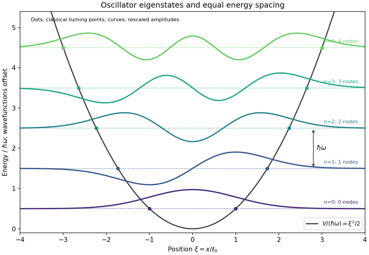
The wavefunctions are plotted with arbitrary vertical scale about their energy levels. Their signed excursions are amplitudes, not additional energies or probability densities.

In the position representation in quantum mechanics, $\hat{\mathbf{p}}=-i\hslash \nabla$. Therefore the orbital angular momentum operator givesAt fixed $r,\theta$, the spherical coordinates obey ${\partial }_{\varphi }x=-y$, ${\partial }_{\varphi }y=x$, and ${\partial }_{\varphi }z=0$. The chain rule consequently gives ${\partial }_{\varphi }=-y{\partial }_x+x{\partial }_y$, henceThe derivative holds the other two spherical coordinates fixed; it is not a derivative along an arbitrary spatial curve.

For a fixed magnitude zero point, photometric magnitude uncertainty follows from propagation of uncertaintyThis is the absolute standard uncertainty of the apparent magnitude. The requested fractional uncertainty is insteadThis is the requested fractional standard uncertainty as a function of $m$; there is no single numerical fractional error independent of the magnitude. At $m=0$ it is undefined. Moreover, its value changes when the magnitude zero point changes; the absolute magnitude uncertainty is the useful invariant of such a zero-point shift. Treating the stated percentage as a finite perturbation rather than a standard uncertainty gives changes $-0.1035$ mag for $f\mapsto 1.1f$ and $+0.1144$ mag for $f\mapsto 0.9f$, consistent with the linear estimate.

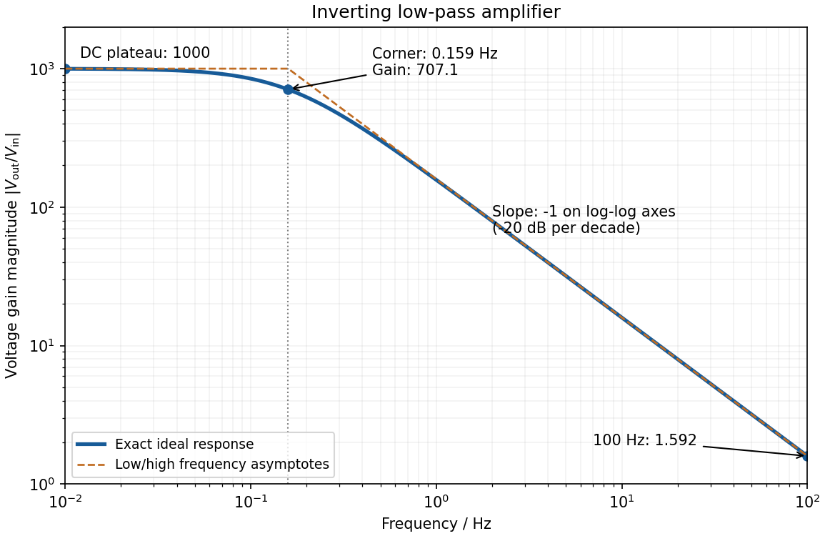
negative feedback and the ideal operational amplifier's virtual short hold the inverting node at zero potential, with no current entering either input. The parallel feedback resistor and capacitor have electrical impedanceKirchhoff's current law at the inverting node gives $V_{\mathrm{in}}/R_i=-V_{\mathrm{out}}/Z_f$. For the component values read from the circuit,This inverting low-pass amplifier has a DC gain magnitude of 1000 and cutoff frequency $f_c=(2\pi R_{f}C{)}^{-1}=0.15915$ Hz. At the corner, $|G|=707.1$. Above it the gain approaches $1/(2\pi f{R}_{i}C)=159.15/f$, with $f$ in Hz: a slope of $-1$ on logarithmic axes, or $-20$ dB per decade on a Bode plot. At $0.01,1,10,100$ Hz the magnitudes are approximately $998,157.2,15.91,1.592$. These are voltage ratios, not decibels.