Some Part IB Physics A and Physics B past papers have solutions alongside them in the restricted teaching system; the specific years have not been verified. Check each paper before selecting it for new solutions, and skip papers with existing solutions.[ref]
The initial table of content was limited to the first level because it is larger than 1000 articles. There are 1197 articles in total. Expand a branch to load its children.
Let the infinite outer walls be at , the finite steps at , and the three potential energy values be . The original drawing specifies the orderingThe energy eigenstates can be chosen real. The Dirichlet boundary conditions are ; wavefunction matching at a finite potential step requires both and to be continuous at . In particular, neither finite step acts as an additional hard wall.
The Time-independent Schrödinger equation givesThus a wavefunction is sinusoidal in a classically allowed region, with wavenumber , and a linear combination of exponential functions in a classically forbidden region, with inverse decay length . Its curvature changes sign relative to at a step crossing ; its slope does not jump.
By the Sturm oscillation theorem, the three energy eigenstates have exactly zero, one, and two interior nodes, respectively. Choose their global phases so that their slopes at the left wall are positive:
- : a positive lobe in the left-hand potential well, followed by a nonoscillatory tail through the barrier and right-hand region. The tail reaches zero at the right wall. There are no interior nodes.
- : two lobes of opposite sign in the left-hand potential well, with one interior node, followed by a nonoscillatory tail of the sign of the second lobe. Both the middle and right regions are classically forbidden regions.
- : sinusoidal behavior in both outer regions, joined through the nonoscillatory barrier. There are two interior nodes in total. The right-hand wavelength is longer than the left-hand wavelength, because .
For , the right-hand piece is proportional to , rather than a pure decaying exponential: this enforces the finite-distance hard wall exactly. The barrier pieces likewise contain both exponential solutions. Their small tails are an instance of quantum tunnelling.
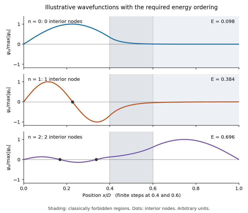
This is an original illustrative calculation, with vertical lines marking only the region boundaries. It uses , , , , , , and in arbitrary energy units. Its lowest energy eigenvalues are approximately , so it has exactly the required ordering. Here both nodes of the third wavefunction happen to lie towards the left; its dominant lobe is on the right. These precise positions and relative amplitudes are illustrative: the original drawing supplies no numerical lengths, barrier heights, or mass, so it does not determine a unique quantitative wavefunction. The required sketch features are the matching, curvature, hard-wall zeros, and ordered node counts.
The protons at the Large Hadron Collider are ultrarelativistic: their energy is much greater than their rest energy, about . The relativistic energy-momentum relation therefore gives . Using the de Broglie wavelength,Thus the conventional de Broglie wavelength estimate is a distance of order .
There is a conventional factor of in interpreting this estimate. Spatial resolution from momentum transfer is often expressed as , where is the transferred momentum multiplied by the speed of light. Taking of order the beam energy givesBoth conventions describe the same characteristic scale up to . The beam energy alone does not give an exact experimental spatial resolution: a particular collision probes a scale set by its actual momentum transfer.
The Born rule uses the squared modulus of the wavefunction, not its real part. Write . ThenWavefunction normalization requiresIntegrating the probability density over the required interval gives the dimensionless probabilityThus approximately of position measurements fall in this interval.
Let denote an incident muon and a detector signal. The selected sample is conditioned on . The law of total probability givesBy Bayes' theorem, the contamination, namely the conditional probability that a selected particle is not a muon, isFor example, per incident particles the expected selected counts are true muons and other particles. The denominator is the selected particles; the rejected muons are outside this sample.
For the fundamental alone, the Nyquist–Shannon sampling theorem places the limiting sampling rate at twice that frequency:Use a rate strictly above this boundary for a sinusoid of unknown phase: exactly two samples per cycle can, for a particular phase, all fall at zero. If higher Fourier harmonics are retained, the sampling rate must instead exceed twice the highest retained frequency, or those components must be removed to prevent aliasing.
For a straightforward discrete Fourier transform estimate, Fourier frequency resolution obeys . Resolving therefore suggestsAt the limiting sampling rate this is about samples. These are the usual sampling and spectral-resolution estimates. The value is not a universal lower bound on single-tone frequency estimation: fitting a sinusoidal model with sufficiently low noise can estimate its frequency more precisely than the spacing of discrete Fourier transform bins. The question gives no noise level or estimator, so a sharper universal minimum time cannot be deduced.
Use the canonical commutation relations , with cross-coordinate commutators zero. For either coordinate,Thus . To obtain the required Hamiltonian, the ratio of its position operator and momentum operator coefficients must be preserved:where the positive root follows from the requested signs. ConsequentlyThe annihilation operators are dimensionless; has units of inverse length and has units of inverse momentum. Operators belonging to different coordinates commute automatically. Writing the number operators as , substitution givesThe constant is the sum of the two zero-point energies of this two-dimensional isotropic harmonic oscillator.
For either number operator , positivity follows fromHence an eigenvalue cannot be negative. The commutatorsshow that , if nonzero, is an eigenstate with eigenvalue . For a normalized eigenstate, .
If were not an integer, successive nonzero lowerings would eventually reach an eigenstate with . Its next lowering would have nonzero norm but a negative eigenvalue, contradicting positivity. The ladder must therefore terminate at , with . Conversely, successive applications of the creation operator never vanish, becauseThe normalizable bottom state exists explicitly: solving gives . Thus the number operator has exactly the non-negative integer eigenvalues.
Since the two coordinate number operators commute, use the product eigenstates . Their energy eigenvalues areAt fixed , the allowed pairs are . Thus the energy level has quantum degeneracy , and the ground-state energy is .
The number operator commutators established above imply that is proportional to and to . Their norms determine the magnitudes of the proportionality constants:Choose the phase of the normalized ground eigenstate once, then define recursivelyThis removes the otherwise arbitrary relative phases of the eigenstates. The Hermitian adjoint relation then fixes the lowering coefficient with the same positive sign, givingAt , the second expression means the zero vector, ; it does not introduce a physical state .
Set . Taking the Hermitian adjoint reverses the order of products, so . Complex conjugation also reverses the sign of , and thereforeThus is a self-adjoint operator on the usual oscillator states.
Using the coefficients in part (a), products containing two position operators or two momentum operators cancel in the difference. Cross-coordinate operators commute, leavingHenceIt is the component of orbital angular momentum perpendicular to the plane, with units (equivalently ). The rotational symmetry of the two-dimensional isotropic harmonic oscillator makes this a conserved observable; directly, each term in preserves , so .
The specified energy requires , so the relevant energy eigenspace has the orthonormal basisApplying the creation and annihilation operators givesThus its matrix in this ordered basis isWriting , the characteristic polynomial gives . The possible angular momentum eigenvalues are thereforeFor completeness, normalized simultaneous energy and angular momentum eigenstates areEach value occurs once in this energy eigenspace. Equivalently, circular ladder operators of a two-dimensional oscillator give and . With , the difference can only be .
For a particle in a ring, the arc-length coordinate is . The tangential kinetic energy isThe constraint removes radial motion; the constant potential energy along the ring can be chosen as zero. The tangential momentum operator is , or equivalently the angular momentum operator is . ThusIts physical domain has periodic boundary conditions, and . These make the Hamiltonian self-adjoint and reflect that and describe the same point. No magnetic flux or additional angle-dependent potential energy is present.
Solving the Time-independent Schrödinger equation with gives . The periodic boundary condition requires , hence . With the angular integration measure , wavefunction normalization givesso a convenient orthonormal eigenbasis isThe ground state is nondegenerate. For each , and span a two-dimensional energy eigenspace; real sine and cosine combinations are an equally valid basis. These opposite-circulation eigenstates have angular momentum and .
If instead the wavefunction is normalized with respect to physical arc length , its expression is . The two conventions describe the same probability, since . The remaining parts use .
Put . The two-particle product energy eigenstates areBecause the particles are distinguishable, and are distinct when . Also, the signs of nonzero integers distinguish opposite angular momenta. The quantum degeneracy is therefore the number of ordered integer pairs at each sum of squares.
The first distinct energy levels are . This ordering matters: is the third excited level, while is the fourth excited level.
These counts concern energy eigenspaces; arbitrary quantum superpositions within each one do not create additional independent states.
Identical spin one-half particles are fermions. By fermionic exchange symmetry, the complete spatial-and-spin wavefunction must change sign when the two particle labels are exchanged. Define the normalized antisymmetric spin-one-half singlet stateand the three symmetric spin-one-half triplet statesThe Hamiltonian is independent of spin, so these spin functions carry no additional energy.
Both particles can occupy if their spin factor is antisymmetric. The unique ground state wavefunction isTwo equal-spin particles could not share this orbital, by the Pauli exclusion principle.
At the first excited energy, , one orbital is and the other is with or . Define symmetric and antisymmetric normalized spatial functionsFor each , all allowed wavefunctions are spanned byThere are orthonormal states, hence first-excited-state degeneracy . In each product, exactly one factor is antisymmetric, ensuring the required total fermionic exchange symmetry.
The original apparatus has two small masses at distance from the suspension axis. Neglecting the rod's moment of inertia, their total moment of inertia is , consistent with the supplied torsion pendulum period. Treat and as exact because no uncertainties are specified. Rearranging the period relation givesThe torsion constant is a restoring torque per unit angle. In dimensional calculations the radian is dimensionless.
Using first-order propagation of uncertainty, with the quoted period uncertainty interpreted as a standard uncertainty,Consequently
Rearrange the given torsion balance equilibrium relation asA useful choice, preserving equal measurement uncertainties on the vertical axis, isWith angle measured in radians, is dimensionless and has units , so has units , as required. The four values, in the order of the original table, areThe corresponding values are , each with standard uncertainty . The uncertainty of is negligible by assumption, making linear regression through the origin appropriate for the proposed model.
All four angle measurements have the same standard uncertainty, so ordinary least squares minimizesDifferentiation givesThus the unique minimum isThe overbars denote sample means over the four observations. Numerically,soThe fixed have negligible uncertainty. Assuming independent errors in the four , propagation of uncertainty in quadrature givesHenceIf the period measurement is independent of the angle measurements, including its calibration uncertainty givesThis last uncertainty includes the stated random measurement errors only. Whether the model describes the data must be checked before treating it as a reliable measurement of the gravitational constant.
Assume independent normally distributed angle errors with known standard deviation . The relevant chi-squared test uses the sum of squared standardized residuals,For the model through the origin, the predictions and residuals, expressed in milliradians, areConsequently . There are statistical degrees of freedom. The upper-tail P-value is approximately ; equivalently the value greatly exceeds the critical value . The zero-intercept model is strongly rejected under the stated errors.
For the alternative linear regression, minimize . Setting both partial derivatives to zero gives the normal equations, whose solution isFor these data , , and . This yieldsThe new predictions are , with residuals . ThereforeThe affine model is compatible with the data. Allowing for its additional fitted parameter, the decrease has a chi-squared distribution with one statistical degree of freedom under the nested zero-intercept hypothesis, corresponding to . Thus the model with a fitted intercept provides the better description, rather than merely lowering the residual by adding a parameter.
With the measurement variance treated as known, the coefficient uncertainties areHence , about standard deviations above zero. A positive constant systematic error in the angular zero, or an additional nearly constant torque, could account for it. Its presence is evidence against the ideal zero-intercept model; four points alone do not identify the physical cause uniquely. A calibration error in only rescales the inferred gravitational constant and cannot remove this residual pattern.
Using the fitted slope after allowing for this offset would give , with the period and slope errors combined in quadrature. This is conditional on the constant-offset model.
Time dependence in quantum mechanics describes how a prepared quantum state changes and thereby changes the probabilities of later measurements. For an isolated system, the Schrödinger picture assigns this evolution to a state vector , governed by the Time-dependent Schrödinger equationThe Hamiltonian is a self-adjoint operator; it has units of energy, while has units of action, so has units of inverse time. For a particle with potential energy , this becomesGiven a suitable initial wavefunction and the physical boundary conditions, this first-order equation determines its subsequent propagation. Its linearity means that the evolution of a quantum superposition is the corresponding quantum superposition of evolved states.
For a real potential energy, this equation and its complex conjugate imply the local continuity equationHere is the probability density and the probability current. Vanishing net boundary flux preserves wavefunction normalization, as required by the Born rule.
The time-evolution operator packages the solution for every initial state:Because , differentiation givesTherefore : this is unitary time evolution, preserving inner products and all state norms. It is reversible, with , and obeys the composition law .
For a time-independent Hamiltonian, the solution is the operator exponentialIf the Hamiltonian varies with time, the analogous simple exponential of its integral is valid when for all relevant times. Otherwise time ordering is essential:The meaning is explicit in the first terms of the ordered series,the later-time operator stands on the left. In the position representation, the same propagation is expressed by the quantum-mechanical propagatorIts initial value is the Dirac delta function .
A time-independent Hamiltonian has energy eigenstates satisfying . A single such initial state evolves asIt is a stationary state: its global phase changes, but its probability density and the distributions of time-independent observables do not. Its energy is sharp. Any quantum superposition entirely within one degenerate energy eigenspace also acquires one common global phase and is stationary. Stationarity does not require zero probability current; for instance, on the ring has a constant density and persistent circulation when .
An arbitrary normalized state can instead contain different energy eigenvalues:A continuous spectrum requires corresponding integrals. For the discrete case, an energy measurement gives with fixed probability (summed over degeneracies), but relative quantum phases change with time. ConsequentlyThe interference terms can oscillate at angular frequencies . For two populated energy levels, this supplies a characteristic period when the interference term is nonzero. Thus fixed energy populations do not imply a stationary spatial distribution.
For a normalized state and an observable , its expectation value isThis is the statistical mean over repeated preparations and measurements. In an eigenbasis of energy eigenstates for a time-independent Hamiltonian and a time-independent ,Only matrix elements connecting different energies can generate these oscillations. If , its expectation value is constant for every initial state, provided it has no explicit time dependence.
Differentiating the expectation value and substituting the Schrödinger equation for both the bra and ket proves the general Ehrenfest theorem:Equivalently,These manipulations require the state to lie in the relevant operator domains. Taking gives , so energy is conserved under a time-independent Hamiltonian.
For , the canonical commutation relation givesHence the particularly useful position-and-momentum form of Ehrenfest theorem isIt resembles Newton's second law, but the mean force generally differs from the force at the mean position. If a narrow wave packet samples a region where the force varies little, gives approximate classical motion. For a quadratic potential energy this replacement is exact. In particular the quantum harmonic oscillator obeysThe centroid follows the classical harmonic oscillator, although this does not specify the full evolving wavefunction or its width.
The Heisenberg picture expresses the same physics by assigning evolution to observables instead:The expectation value is unchanged, and differentiation yields . Thus state propagation, evolving expectation values, and the classical correspondence in Ehrenfest theorem are mutually consistent descriptions of the same unitary time evolution.
Use Fresnel diffraction, since the detector moves along the axis through successive near-field interference extrema. Write for its distance from the opening and for the integration coordinate within the opening. For a uniform incident plane wave, the on-axis complex amplitude, in the paraxial approximation, is proportional toThus the light intensity relative to the incident value isThe Fresnel number is an odd integer at a maximum and an even integer at a minimum. It decreases as the detector moves away. Adjacent extrema therefore differ by one:ConsequentlyAs a check, at and at , so these are indeed a maximum followed by the next minimum. Also , consistent with the paraxial approximation.
The components are in phase quadrature when the axes of the ellipse coincide with the coordinate axes. Since the wave amplitude is one and the wave amplitude is two, the Jones vector must have .
A handedness convention is essential. Adopt the optical convention in which right-handed elliptical polarization rotates clockwise when viewed toward the source, from the positive- side. With the paper's phase convention for complex amplitudes, this givesThe tip follows . In particular,
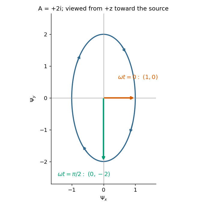
The figure states the viewing direction and shows increasing time. Under the alternative convention that calls rotation from toward right-handed when looking along propagation, the equally consistent answer is and the second vector is . The original paper does not state a handedness convention, so its wording alone cannot select between these labels; the real components and viewing direction remove the ambiguity.
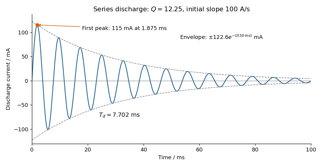
Choose positive electric current in the initial discharge direction, since the source diagram does not label the initial plate polarity or a current arrow. Let be the charge remaining on the initially positive plate, so . Kirchhoff's voltage law for the series RLC circuit givesThe natural angular frequency, damping coefficient and quality factor areSince (equivalently ), this is an underdamped RLC response. With , satisfying the initial conditions givesand differentiating givesThe electric current starts at zero with . Its wave period is , its zeros occur every , and its positive and negative wave envelopes decay with time constant . The first maximum obeys and is at . The electric current tends to zero as the initial capacitor energy is dissipated in the resistor.
Take a p-n junction made from one semiconductor, with the p-type semiconductor on the left and the n-type semiconductor on the right. At thermal equilibrium the chemical potential is horizontal throughout. Before contact the chemical potential lies nearer the valence band on the p side and nearer the conduction band on the n side; after contact the band edges bend to permit one common value.
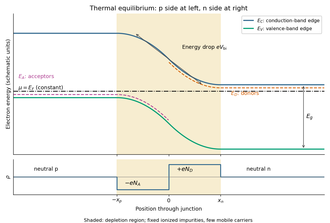
Original equilibrium p-n junction energy band diagram, impurity levels, common chemical potential and depletion region
. Details. In this orientation both the conduction band edge and the valence band edge decrease from p to n by . For a homojunction their separation is constant. The acceptor impurity level lies just above where acceptors are present, and the donor impurity level lies just below where donors are present. These impurity levels follow the local band bending; they do not form one additional horizontal band across the device.
The shaded depletion region has few mobile Electrons or electron holes and contains fixed negative ionized acceptor impurities on the p side and positive ionized donor impurities on the n side. Thus its electric field points from n to p. Its neutral outer regions have negligible electric field, so the band edges become flat there. In the depletion approximation, charge neutrality requires ; the symmetric drawing illustrates rather than assuming that equality is universal. Diffusion and field-driven drift current cancel at equilibrium: no applied voltage does not mean zero internal electric field or zero built-in electric potential difference.
In an ordinary three-dimensional crystalline electrical insulator, heat is carried mainly by phonons. Kinetic theory gives the estimatewhere is heat capacity per unit volume, is a typical sound speed, and is the phonon mean free path. The thermal conductivity has units .
At low temperature, , the Debye model gives . With phonon-phonon collisions frozen out, diffuse scattering at the sample boundaries makes approximately constant, and is nearly constant. HenceAt high temperature, of order or above the Debye temperature, the Dulong-Petit law makes approximately constant. Anharmonic phonon scattering, especially resistive Umklapp scattering, has a collision rate approximately proportional to . Thus andThese two regimes usually give an intermediate maximum of thermal conductivity. The assumptions matter: glassy materials, strong defects or specular boundary reflection can change the low-temperature law; these are not universal laws for every electrical insulator.
A nondispersive wave has a linear dispersion relation over the relevant range, so every Fourier transform component has the same phase velocity and group velocity . A wave packet then translates without spreading in an ideal homogeneous lossless medium.
For wave dispersion, depends on frequency or wavenumber. Different components accumulate different phases, and in general the group velocity differs from the phase velocity; variation of group velocity across the spectrum produces spreading of a wave packet. The membrane material can be nondispersive while confinement in a membrane waveguide introduces wave dispersion along its length.
Twice differentiating the proposed normal mode givesIt therefore solves the two-dimensional wave equation precisely whenThe fixed-edge boundary conditions require . The first is automatic, and the second requires . The nonzero normal modes are thereforeThe apparent choice gives identically zero displacement for this sine solution. There are no imposed end conditions in , so is continuous rather than quantized by a second length. For a propagating mode it is real; the plus sign in the stated convention describes propagation in . Each positive integer labels a transverse standing wave across the strip.
For a fixed transverse normal mode, define its cutoff angular frequencyThe longitudinal phase velocity and group velocity, for propagation in , areThus , and . The large longitudinal phase velocity reflects the geometry of the transverse standing wave and does not imply faster transport of energy than the membrane wave speed.
The cutoff frequency of a membrane waveguide for mode isAt cutoff and ; the longitudinal phase velocity has no finite value. Below cutoff,and a bounded field excited at decays as . It is an evanescent wave, rather than a freely propagating mode carrying net time-averaged energy flux down an indefinitely long uniform strip. A finite section can still transmit through coupling of evanescent fields.
The natural interpretation is the fundamental transverse normal mode, . Indeedso only propagates over the main part of the given Gaussian distribution of angular frequencies. Its centre travels atDifferentiate the group velocity with respect to angular frequency:At the centre this is . The one-standard-deviation group velocity spread is consequentlyOver the central travel time the associated spatial shear isEquivalently, use representative components at , for which and . Their separation after isAt a fixed detector away, the corresponding arrival-time difference is .
The paper asks for an estimate of spreading, without specifying a spatial width convention or the initial spectral phase. A Gaussian distribution has no finite full range. Thus is a one-standard-deviation dispersive contribution, whereas about describes the separation of the representatives. Neither is automatically the increase in the packet's original width. For an initially unchirped Gaussian wave packet in the narrow-band approximation, independent initial and dispersive contributions combine as ; a packet with an initial chirp can behave differently. The modal assumption and width convention must accompany the numerical answer.
Different transverse normal modes have different cutoff frequencies and group velocities. A pulse exciting several of them reaches the output in delayed modal components, causing intermodal dispersion, pulse distortion and overlap of successive signals. Their interference also makes the transverse wave intensity pattern depend on propagation distance; irregularities can transfer energy between modes.
Mitigations are to operate between the first and second cutoff frequencies of a membrane waveguide, excite only the desired mode shape with a suitable source, and use smooth uniform boundaries or gradual transitions to reduce mode conversion. Reducing the signal bandwidth keeps its spectrum inside the single-mode interval and reduces group velocity dispersion within the selected mode. Single-mode operation removes intermodal dispersion but does not remove the dispersion derived in part (b).
For the normally incident plane wave, the incident complex amplitude and phase are uniform across the aperture. Treat the field using scalar diffraction, with the aperture represented by its prescribed amplitude transmittance . Let be the distance from the aperture centre to the observation point and let be the transverse direction cosines of that point.
Across an aperture of characteristic size , the Fraunhofer diffraction assumptions are that , so and the obliquity factor is nearly constant, and that the quadratic contribution to the propagation phase is negligible:The remaining path-length dependence is linear:A coherent monochromatic wave and an aperture large enough relative to wavelength for the scalar aperture model complete the usual physical assumptions. The complex amplitude becomeswhere includes the common propagation phase, distance factor and nearly constant obliquity factor. For the central part of a planar screen in the paraxial approximation, and . Small observation angles are useful for that screen-coordinate formula; a general far-field Fourier transform can instead use the exact direction cosines. A lens can also produce this pattern in its focal plane without requiring a physically very distant screen.
The far-field complex amplitude is the two-dimensional Fourier transform of the aperture amplitude transmittance, evaluated at transverse spatial frequencies , . The light intensity is proportional to the squared magnitude of this transform.
Use linearity to add the transforms of simpler aperture components, preserving their relative phases. A translated component acquires a complex exponential factor. Repeated identical openings can be expressed as the convolution of one opening with a sum of Dirac delta functions; the convolution theorem then factors the field into a single-opening transform and an array factor. Multiplying aperture functions instead convolves their transforms. These operations simplify complex apertures without repeatedly evaluating the full diffraction integral. It is the complex amplitudes, rather than their wave intensities, that are added for coherent illumination.
Take the quoted separation to mean adjacent slit centre spacing . For three equal very narrow slits at , the Fraunhofer diffraction complex amplitude in the transverse direction isWith denoting one narrow slit's contribution, the light intensity isThe quotient is interpreted by its limit where both numerator and denominator vanish. At small angles on a screen at , and . Principal interference fringes occur atBetween successive principal maxima there are two zeros, at and . Halfway between them is a smaller maximum , one ninth of a principal peak. The pattern is symmetric about . The positions quoted in millimetres use the paraxial approximation; exactly and .
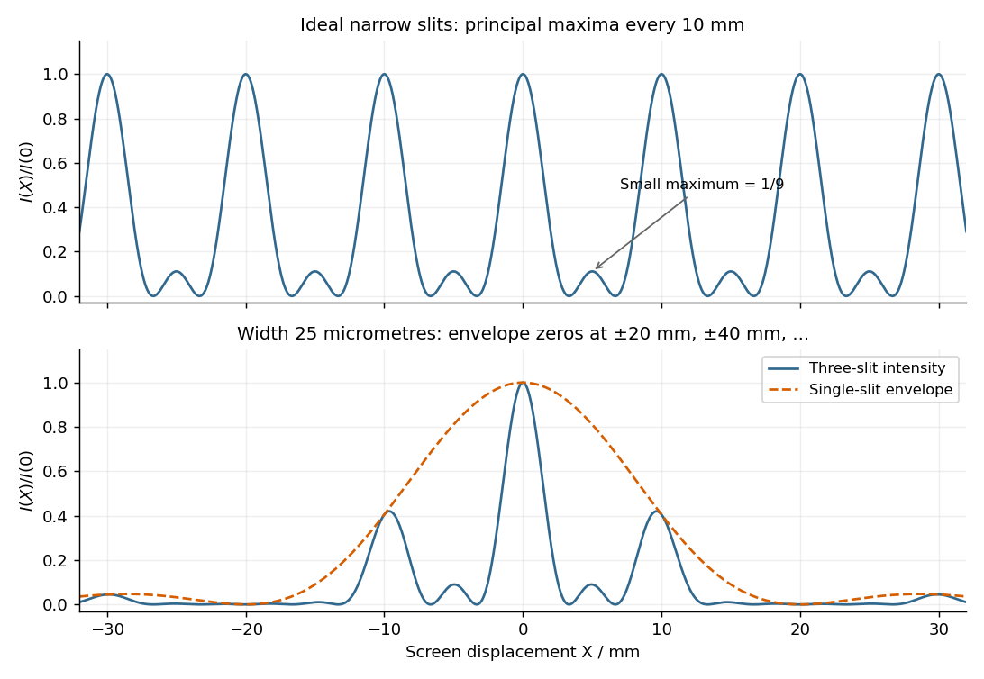
Original calculated Fraunhofer diffraction patterns for three narrow slits and for three finite-width slits
. Details. A slit of width has the single-slit diffraction complex amplitude factor , where . Thus for ,The interference factor keeps the same zeros and the same nominal principal-order positions as in part (i), while the single-slit diffraction wave envelope suppresses off-axis wave intensity. Its zeros areAt nominal principal diffraction orders , the wave envelope factor is . ConsequentlyAll nonzero even principal orders are missing. The central single-slit diffraction maximum extends between the envelope zeros near and includes the central and the principal orders. Because there are only three slits, the maxima of the product can shift slightly from the nominal nonzero-order positions; the quoted values are the exact product at those positions. The lower panel of the figure shows the full product.
Both panels normalize to their own central wave intensity. An absolute comparison would require the unspecified widths and transmitted power of the initially “narrow” slits; the normalized pattern change is fully determined.
For equally spaced illuminated slits, with , summing a geometric series of complex amplitudes givesHere is the one-slit single-slit diffraction wave envelope. The grating equation for principal maxima iswith height and much weaker subsidiary maxima between orders. The first zeros around order are , so the angular distance from a maximum to its first minimum is, for large ,Changing wavelength by moves the same diffraction order byThe Rayleigh criterion places the maximum for one wavelength at the first zero for its neighbour. Equating these separations givesThis is the ideal resolving power of a diffraction grating, for an illuminated and transmitted order with sufficiently narrow source and instrumental broadening. The zeroth order has no wavelength separation and therefore no useful spectral resolving power. The distinction between and the span of the outer slit centres is a small edge convention; the exact state count in the resolving-power formula is .
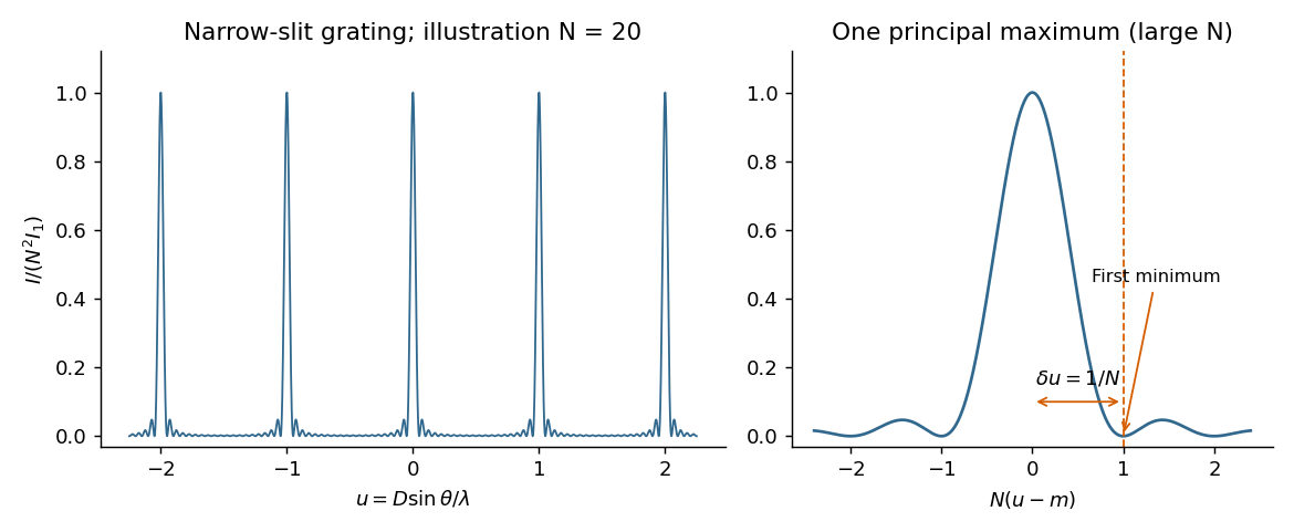


The required resolving power of a diffraction grating isFor illuminated slits, . In orders , the ideal resolvable wavelength differences are respectively , , and . ThusFourth order gives , only a modest margin. It must also exist: for normal incidence the grating equation requires , with needed to avoid an exactly grazing order. The relevant order must transmit appreciable light intensity rather than lie at a single-slit diffraction zero, and the source and detector widths must preserve this resolution.
The original question gives only the slit count, not the line spacing, slit width, usable diffraction order or instrumental broadening. It therefore supports the conditional conclusion “yes in fourth or higher usable order”, but not an unconditional historical claim that this particular instrument resolved the sodium absorption line doublet in its observed configuration.
For a plane wave wavefunction , impose the cyclic or periodic boundary condition . It requiresAdjacent allowed wavenumbers on the full signed axis are spaced by . Ignoring spin, the density of states per unit is consequentlyBoth positive and negative are included in this density. It is not yet the density per unit magnitude , which has an extra factor of two away from zero. In independent dimensions the same periodic boundary conditions give one spatial state per -space cell of measure .
To preserve the convention of part (a), first count one spin species. Define as the number of spatial states in the whole specimen in that energy interval. PutIn one dimension there are intervals near both and , so the one-dimensional free-electron density of states isThus . The factor of two here comes from opposite momenta, not spin. For physical Electrons with two spin states, the spin-summed density of states is . These expressions are continuum approximations away from individual discrete levels.
In two dimensions the density of states in space per spin species is . A annulus of radius and thickness has area . ThereforeThe two-dimensional free-electron density of states is constant in energy, , above the band bottom. Including both spin states gives . Dividing by gives the density per unit physical area, rather than the total specimen's density.
In three dimensions use the -space density of states per spin species and the spherical shell volume :Thus the three-dimensional free-electron density of states grows as . For physical Electrons, including both spin states givesAll three total density of states functions have units when energy is in joules; they count states per energy interval. The paper explicitly suppresses spin in (a) but does not repeat that convention in (b), so giving both conventions avoids a hidden factor-of-two ambiguity. Parts (c)--(f) below use the physical two-spin-state electron gas.
Articles were limited to the first 100 out of 1197 total.
Articles by others on the same topic
There are currently no matching articles.