Original source: Released examination PDF, physical pages 100–105. All alternatives are treated below.
The Born rule uses the squared modulus, so the imaginary term contributes positively: . For , wavefunction normalization would multiply the supplied expression by . Equivalently, take the ratio of the integrals directly:Using instead of would fail to produce a real, nonnegative probability density.
For the quantum harmonic oscillator, put and . The normalized energy eigenstates arewhere is a Hermite polynomial. Successive energies are equally spaced; the ground state retains zero-point energy . The th wavefunction has nodes of a wavefunction and parity . In particular, the first three shapes are proportional to , , and . The classical turning points satisfy ; the wavefunctions extend beyond them and decay, rather than ending abruptly.
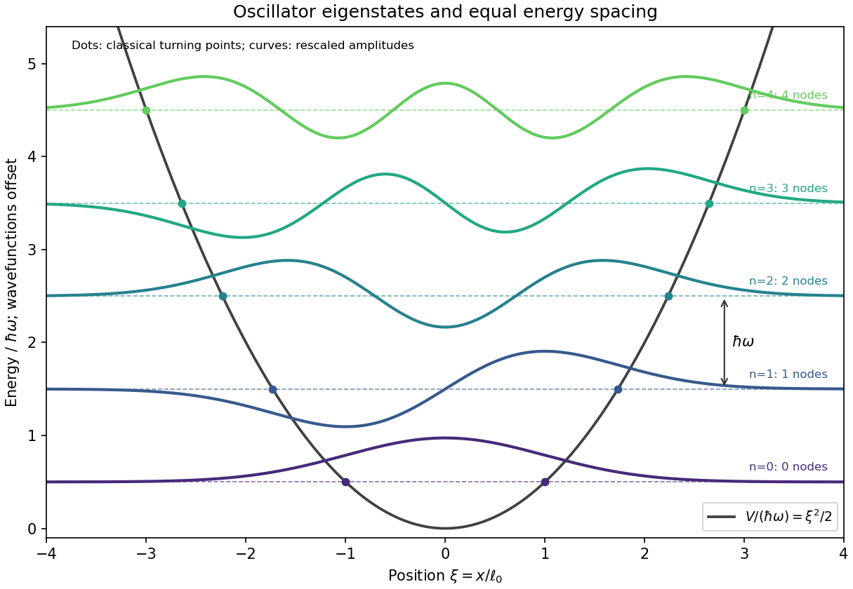
The wavefunctions are plotted with arbitrary vertical scale about their energy levels. Their signed excursions are amplitudes, not additional energies or probability densities.
In the position representation in quantum mechanics, . Therefore the orbital angular momentum operator givesAt fixed , the spherical coordinates obey , , and . The chain rule consequently gives , henceThe derivative holds the other two spherical coordinates fixed; it is not a derivative along an arbitrary spatial curve.
For a fixed magnitude zero point, photometric magnitude uncertainty follows from propagation of uncertaintyThis is the absolute standard uncertainty of the apparent magnitude. The requested fractional uncertainty is insteadThis is the requested fractional standard uncertainty as a function of ; there is no single numerical fractional error independent of the magnitude. At it is undefined. Moreover, its value changes when the magnitude zero point changes; the absolute magnitude uncertainty is the useful invariant of such a zero-point shift. Treating the stated percentage as a finite perturbation rather than a standard uncertainty gives changes mag for and mag for , consistent with the linear estimate.
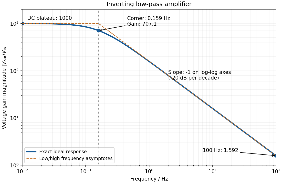
negative feedback and the ideal operational amplifier's virtual short hold the inverting node at zero potential, with no current entering either input. The parallel feedback resistor and capacitor have electrical impedanceKirchhoff's current law at the inverting node gives . For the component values read from the circuit,This inverting low-pass amplifier has a DC gain magnitude of 1000 and cutoff frequency Hz. At the corner, . Above it the gain approaches , with in Hz: a slope of on logarithmic axes, or dB per decade on a Bode plot. At Hz the magnitudes are approximately . These are voltage ratios, not decibels.
Single travelling wave. Differentiation of the plane wave gives , so its probability current isThis is probability density times the free-particle velocity .
Counterpropagating waves. Remove the common time phase and set . Direct multiplication givesConsequentlyThe interference term is purely imaginary in the last real-part operation. The probability density can have interference fringes even though this net probability current is spatially constant.
Scattering amplitudes. Locate the step at and first take . With and , useThe common factor has been suppressed. A finite step with the same mass on both sides requires continuity of and , giving and . HenceIf , choose , , so the transmitted wave decays. The same amplitude formulae continue to hold, but the semi-infinite forbidden region carries no outgoing probability current: and .
Flux balance. In the propagating case,In particular,The velocity ratio in is essential: the squared transmission amplitude alone is not the transmission probability when the two velocities differ.
Numerical transmission. The mass cancels from the ratio, and the energies can remain in the same electronvolt units:Thus about is transmitted and reflected, despite the incident energy exceeding the step.
Stationary states. Inside the infinite square well, the time-independent Schrödinger equation has sinusoidal solutions. The boundary conditions select ; normalization then givesEach wavefunction vanishes outside the well. There is no nonzero state.
Immediate energy measurement after expansion. For the one-sided sudden expansion of an infinite square well, take the original wall at as fixed, so the expanded well occupies . In the sudden approximation, the initial wavefunction remains on , extended by zero elsewhere. The new ground state is . Its probability amplitude isThe Born rule therefore givesThe motion of the walls matters: a symmetric expansion about the old midpoint would instead give . The stated width alone does not explicitly identify the final endpoints. The first result uses the natural continuation of the specified left boundary; if both boundaries are moved, the final location must be supplied. For a new well containing , the overlap is .
Evolution of one energy eigenstate. For a time-independent Hamiltonian operator, write . Substitution into the Time-dependent Schrödinger equation gives , soOnly a global phase changes, leaving all measurement probabilities unchanged.
Delayed energy measurement. Expand the unchanged initial state in the complete new energy eigenbasis,For the fixed-left-wall geometry, direct overlap integration givesorthogonality isolates the new ground-state amplitude as . Its phase cancels on squaring, so the ground-state probability remains for every delay, provided the expanded well remains fixed and no intervening measurement or environment changes the state. The position probability density generally evolves because different eigenstates acquire different relative phases.
Factorization. Put and use the canonical commutation relation :It follows thatThe arises from quantum operator ordering; treating and as commuting would lose the zero-point energy.
Raising the energy. If , thenThus the creation operator produces an energy eigenstate with energy . It is nonzero: for a normalized physical oscillator eigenstate, . Normalize by this norm if a normalized state is wanted.
Lowest wavefunctions and orthogonality. In the position representation in quantum mechanics,The annihilation condition therefore gives . Applying to its solution givesTheir inner product is proportional to , since the integrand is odd. These are the even and odd lowest wavefunctions shown in A2, with energies and .
Exchange constraint. Exchange of two identical particles cannot change physical predictions. For the usual three-dimensional bosonic or fermionic state space, the exchange operator obeys , so its allowed eigenvalues are . bosons use the symmetric overall wavefunction, ; fermions use the antisymmetric overall wavefunction, . Exchange includes the spatial coordinates and all internal labels. The identity alone does not prove which particle species has which statistics; that assignment is the Spin-statistics theorem.
Factored fermion states. If and both factors have definite exchange symmetry, their exchange signs must multiply to . Thus a symmetric spatial factor requires an antisymmetric spin factor, and an antisymmetric spatial factor requires a symmetric spin factor. For two spin-one-half particles, the former spin factor is the singlet ; the latter factors are the three triplet states. A more general entangled spin-space state need not factor, but must still be antisymmetric overall.
hydrogen spin isomers. The two protons are identical spin-one-half fermions. parahydrogen has total nuclear spin , the antisymmetric singlet; orthohydrogen has , the symmetric triplet. Here is a spin quantum number, distinct from the moment of inertia used below.
Rotational restriction. In the electronic and vibrational ground state, these two factors are symmetric under nuclear exchange. Exchanging the protons reverses the internuclear axis, . The spherical harmonic rotational state contributes the exchange sign . Overall antisymmetry therefore requiresHence parahydrogen has even ; orthohydrogen has odd . The here labels molecular rotation, rather than the angular momentum obtained by also coupling the nuclear spins.
Conversion heat. The ortho-para conversion heat follows from the linear rigid rotor approximation, with . Thus conversion of one molecule from to releasesNeglecting the small electron contribution to the molecular mass, a sample of mass contains molecules. Only the initial orthohydrogen fraction releases this energy, givingThe estimate uses pm, kg and J s. Handbook-level rounding and the rigid rotor approximation justify about three significant figures, not a high-precision thermochemical prediction.[ref]
Storage consequence. The internal conversion is a delayed heat source even in a well insulated container, causing warming or additional evaporation of the liquid. Insulation reduces external heat transfer but does not remove this source. Converting to predominantly parahydrogen during liquefaction, while removing the released heat, reduces the subsequent storage heat load. No evaporation fraction can be calculated without a latent heat and a model for how the heat is removed.
A density operator describes both a quantum state prepared in one pure state and a statistical preparation whose members occupy different pure states. If normalized vectors occur with probabilities , defineThe resulting operator is Hermitian, positive semidefinite and has trace one. Positivity follows because . Conversely, the spectral theorem gives such a representation of any finite-dimensional operator with these properties, using its eigenvectors and eigenvalues. The matrix representing depends on the chosen basis; the operator and its predictions do not.
One operator gives every measurement probability. For a projective measurement with orthogonal projections and outcomes ,For example, the first formula follows by averaging over the preparation. The trace expression is basis independent. A general measurement replaces by positive measurement effects that sum to the identity, without changing the probability formula. Thus specifies the statistics accessible to measurements on that system.
The distinction between pure and mixed states is especially transparent in the eigenvalues. A pure state has , , and . A mixed state has at least two positive eigenvalues and . For a qubit,pure states lie on the Bloch sphere; mixed states lie inside the Bloch ball. The maximally mixed qubit can be prepared by choosing equally between the two spin eigenstates, or equally between the two spin eigenstates. These ensembles are different preparation procedures but give the same density operator. No measurement on the resulting qubit alone can identify which ensemble was used.
quantum coherence must be distinguished from merely having two populated levels. In the basis, the state hasBoth give equal probabilities for the two outcomes. A measurement along gives the positive result with probability one for the first state and one half for the second. The off-diagonal entries encode the relative phase information responsible for this difference. Whether a matrix entry is off diagonal is basis dependent; purity is not.
For an isolated system, each component evolves with the same unitary time-evolution operator. Therefore andUnitary evolution preserves the eigenvalues and purity of . A density operator commuting with a time-independent Hamiltonian operator is stationary. A thermal equilibrium example is the canonical ensemble , where and . expectation values then reproduce quantum statistical mechanics without assigning the system a definite energy eigenstate on every run.
A mixed state can also arise without classical randomness in the joint preparation. For a bipartite quantum system, the reduced density operator gives every measurement probability accessible to subsystem . For the Bell state , the joint state is pure, whereas . Its local mixedness reflects entanglement with the inaccessible system; the partial trace discards correlations that matter for joint measurements. More generally, interaction with an environment can suppress off-diagonal entries in a selected basis, producing decoherence while the combined system still evolves unitarily.
Finally, state evolution conditional on a measurement outcome differs from isolated evolution. An ideal projective measurement yielding updates the state by the Lüders rule . Discarding the outcome gives , which generally removes coherence between different eigenspaces. The Von Neumann entropy quantifies mixedness: it vanishes for pure states and reaches for . Multiplying by gives thermodynamic entropy units. These uses make the density operator a common language for preparation uncertainty, measurement, thermal states and entangled subsystems, while retaining their distinct physical origins.
With two coherent paths, the probability amplitude at a screen is . The Born rule givesThe final term shifts when the relative phase changes, producing interference fringes. For slit separation in the far field, the phase difference is approximately ; constructive interference occurs at . Finite slit widths add a diffraction envelope, so an ideal equally bright, infinitely narrow slit model does not predict the full observed envelope.
single-electron interference pattern buildup starts with isolated localized detector events at sufficiently low source intensity. Repeated events accumulate the interference probability distribution. Thus detection is discrete while propagation is described by coherent probability amplitudes. The effect cannot be explained by interference between different particles if the apparatus is occupied by at most one particle at a time. A motivating realization used a field-emission electron source, an electron biprism to recombine two paths, electron lenses and a position-sensitive electron counter; it recorded individual arrivals building up the fringes. This was a biprism realization of two-path interference, not a plate with two literal slits.[ref]
Demonstration of single-electron buildup of an interference pattern by Akira Tonomura and others. section III, American Journal of Physics 57, pp. 117–120
The crucial comparison is between both coherent paths open and a preparation that supplies which-path information. If the paths become correlated with detector states , the joint state is . Ignoring that detector multiplies the interference term by . Orthogonal detector states remove the term completely, while identical detector states preserve it. This is a consequence of entanglement and the partial trace; a human need not read the detector.
In a real test, check the single-path distributions, detector background, source coherence and stability of the relative phase. Classical phase drift can wash out fringes without supplying which-path information. Conversely, localized detections alone do not establish coherent two-path propagation; the controlled phase dependence of their accumulated distribution provides the discriminating evidence.
orbital angular momentum generates spatial rotations and is . With , its components satisfyThus and one component, conventionally , have simultaneous eigenstates, while all three components cannot generally have sharp values. On ordinary single-valued spatial wavefunctions,The spherical harmonics form an orthonormal angular basis. The integer restriction is specific to orbital wavefunctions; half-integer spin is an intrinsic degree of freedom, not the angular dependence of a scalar spatial wavefunction.
The angular momentum ladder operators obeyThe ladder ends at , producing states. A state with specified has a sharp projection , but the angular momentum magnitude is , not . No classical picture of a vector with simultaneously fixed Cartesian components reproduces all these measurement properties.
In a central potential, rotational symmetry gives . separation of variables yields . The radial Schrödinger equation includes a centrifugal potential , which suppresses small-radius amplitude for nonzero . The energy is independent of when rotational symmetry is intact, but need not be independent of . A magnetic field can break that degeneracy. Spatial inversion gives , connecting orbital angular momentum to parity and to the even/odd rotational restriction for the hydrogen spin isomers.
For a nonrelativistic spinless particle in a scalar potential, the Time-dependent Schrödinger equation isAn initial wavefunction together with boundary conditions specifies the evolution. The Hamiltonian operator must be self-adjoint on the appropriate domain for closed-system evolution to be unitary. The equation is linear, so a superposition of solutions is another solution. Its complex wavefunction predicts probability amplitudes; the Born rule separately supplies the connection to measurement probabilities.
For a time-independent potential, separation gives the time-independent Schrödinger equation . Normalizability and boundary conditions select the allowed energies of bound states; scattering states instead use incoming and outgoing boundary conditions and generalized normalization. A general state is a superposition of energy eigenstates, with a spectral integral as well if there is a continuous spectrum. Different energies accumulate different phases, allowing time-dependent position densities and oscillatory expectation values even though a single energy eigenstate has a stationary density.
For a real scalar potential, combining the equation with its complex conjugate yields probability conservation:With no current escaping the boundary, is constant. Matching conditions at a finite potential step follow from the differential equation and enforce the flux balance used in B6.
The Schrödinger equation is a dynamical postulate of nonrelativistic quantum mechanics, not a consequence of classical mechanics alone. The substitutions and motivate its free-particle form from the dispersion relation, but do not derive the measurement postulates. The scalar equation omits intrinsic spin and relativistic particle creation. Spinful or relativistic problems require the corresponding extended theory. Nor does its deterministic unitary evolution, by itself, prescribe conditioning on a particular observed measurement outcome.
Graph. The original plot below places distance on the horizontal axis and recession speed on the vertical axis. Both axes include the origin, so the proportional model and departures from it can be judged directly. The displayed line is the fitted through-origin line, not a sequence joining adjacent observations.
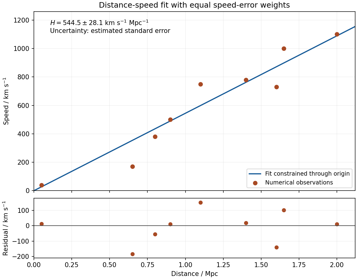
Minimization. Write and . Differentiating the specified chi-squared objective givesThus the unique least-squares minimum isConsequentlyAn unweighted average of would not minimize this chi-squared objective: equal speed errors give greater slope information to the more distant points. No intercept is fitted because the supplied model constrains it to zero.
Estimated error. For the residual estimate of slope uncertainty through the origin, independent equal-variance speed errors implyEquivalently, completing the square gives . The common is not supplied. Estimate it from the residuals, using eight residual degrees of freedom after fitting one parameter:The estimated standard error is km s kpc, givingwith the uncertainty interpreted as one estimated standard error. If the common errors are Gaussian, has a Student's t-distribution with eight degrees of freedom; an exact confidence interval uses the corresponding quantile rather than treating the estimated as known. The quoted error is conditional on exact distances, independent constant-variance speed scatter and the proportional model. A common distance-calibration bias or correlated velocities would not be captured by this residual calculation.
A systematic error is a reproducible displacement caused by the apparatus, procedure or measurement model. Repeating the same experiment can determine its mean very precisely while retaining that displacement. Reducing random measurement error therefore does not establish accuracy.
Start with a measurement model listing the response, zero offset, calibration scale and relevant environmental corrections. Compare the instrument with traceable standards at several points across its working range; a single zero check cannot reveal a gain error or nonlinearity. Measure blanks and backgrounds using the same acquisition chain as the signal. Repeat calibration before and after the run to detect drift, and retain the uncertainty of every applied correction.
systematic-error cancellation by reversal separates a wanted effect from an offset with a different symmetry. For example, a resistance measurement with thermoelectric offset gives and . The difference givescancelling a stable offset, while diagnoses it. Alternate the current direction quickly enough that the offset is approximately unchanged. This does not cancel a current-scale calibration error or resistance changes from Joule heating; vary the current magnitude and monitor temperature to test those effects. Control measurements must target the actual proposed bias.
Randomizing the order of settings prevents slow drift from consistently imitating a physical trend. Interleaving a reference measurement helps track that drift. Reversing geometry, exchanging matched detectors and changing alignment can expose effects tied to one part of the apparatus. Repeating the measurement with an independent method is particularly valuable when its dominant biases differ; agreement between two instruments sharing the same calibration does not test a common calibration error.
Apply justified corrections, propagate their uncertainties and include correlations when the same calibration enters several observations. A systematic component shared by all observations does not shrink as . A measurement uncertainty budget should distinguish the physical origin of each effect from the method used to evaluate its uncertainty: statistical Type A and other Type B evaluations do not simply mean random and systematic, respectively.[ref]
Guidelines for Evaluating and Expressing the Uncertainty of NIST Measurement Results by Barry N. Taylor and Chris E. Kuyatt. sections 2–5 and Appendix D.1.1.6: systematic error and correction
Bayes' theorem updates a hypothesis using observed data. For mutually exclusive exhaustive hypotheses and data of nonzero probability,The prior describes information before these data; the likelihood describes the sampling model; the denominator is the evidence; and the posterior is the updated probability. likelihood and posterior are different conditional quantities. For a continuous parameter, sums become integrals and the posterior is a probability density.
Consider a counter registering independent events at unknown constant rate , observed for known exposure with negligible background and dead time. The observed count has a Poisson distribution:Take a proper gamma prior in shape-rate convention,Multiplying by the likelihood adds the count to the shape and the exposure to the rate. Normalization therefore givesHere has exposure units. This is Poisson-gamma conjugacy. Successive independent counting runs update the same posterior by adding their counts and exposures, so the result agrees with analysing all the data together.
A credible interval contains a specified posterior probability for , conditional on the chosen prior and model. For low counts, the posterior can be asymmetric and sensitive to the prior, and a symmetric Gaussian error bar can be misleading. For large and an exposure dominating prior information, the mean approaches and its standard deviation approaches . Background, missed events or time-dependent rates require a richer likelihood; Bayes' theorem cannot compensate for an incorrect physical counting model. The prior must be specified independently of the same data being used in the likelihood, unless its estimation is explicitly included in a larger model.
shot noise arises from fluctuations in discrete transfer events. For equal charges arriving independently with a constant Poisson rate , the charge collected during is , withThus the relative counting uncertainty is . Longer integration improves the precision of the mean current even when the microscopic arrivals remain irregular.
In the frequency range where independent arrivals can be treated as instantaneous pulses, the one-sided current power spectral density isFor an ideal unit-gain rectangular bandwidth , this gives . boxcar averaging of Poisson shot noise over duration has effective noise bandwidth , reproducing the counting result . The two-sided spectral convention instead assigns to each sign of frequency. Stating that convention prevents a factor-of-two error.
A photodiode illuminated at a stable rate provides a useful measurement: subtract the mean current, amplify its fluctuations through a calibrated linear filter, and compare the variance with the mean photocurrent. Independent detected photoelectrons predict a variance proportional to mean current. Measure the dark and amplifier backgrounds separately, check the filter's effective noise bandwidth and vary illumination to distinguish this term from classical intensity noise, whose variance can scale quadratically with mean current. The shot noise model concerns counting statistics, whereas thermal electrical noise can exist in an unbiased resistor. Walter Schottky's motivating analysis treated amplifier limits and independent electron transfers in thermionic discharge tubes.[ref]
Über spontane Stromschwankungen in verschiedenen Elektrizitätsleitern by Walter Schottky. Part II, especially pp. 557–563
The Poisson result is a model, not a universal consequence of charge quantization. Correlated arrivals, detector dead time, avalanche multiplication or a non-Poisson light source can change the fluctuations. Filtering reduces integrated noise at the cost of temporal resolution. Increasing the detected event rate reduces relative shot noise but raises its absolute variance; balanced photodetection cancels shared classical fluctuations, not the independent shot noise of two uncorrelated detectors.
Original paper: PHYSICS A (2), 28 May 2015; physical PDF pages 106–111.
The photon relation gives . The diffraction-limited angular scale of an aperture of diameter is thereforeFor a uniformly illuminated circular aperture, the Rayleigh criterion instead gives . Both express the same requested estimate. This is an ideal diffraction limit, conditional on the effective diameter behaving as a coherent imaging aperture; photon energy and diameter alone do not specify the performance of a practical gamma-ray telescope.
At distance , the small-angle approximation gives . Thus the transverse resolution is approximately , or with the circular-aperture Rayleigh criterion. This is a transverse separation at the source, rather than a determination of its distance along the line of sight.
Let be the common tension and the linear mass densities. The characteristic impedance of a stretched string is . Continuity of displacement and transverse force at a massless junction gives and . ConsequentlyThe reflected power is . The minus sign of represents a phase reversal, not negative power. Both incident and reflected waves travel in the first string, so their power ratio is simply the squared displacement-amplitude ratio. As a check, and .
Compare a directly transmitted ray emerging at with a ray that makes one extra round trip inside the Fabry–Pérot interferometer and emerges at . Both emerge parallel at angle to the plate normal. The extra internal distance is , and their emergence points differ laterally by . The first ray has already travelled towards a common outgoing wavefront when the second reaches . The air-gap optical path difference in a Fabry–Pérot interferometer follows because optical path length equals geometric path length in the air-gap approximation:The subtraction is essential: comparing distances only inside the plates would compare different outgoing wavefronts. The corresponding propagation phase difference is . Coating reflection phases can add a separate phase offset; they do not change this geometric optical path difference.
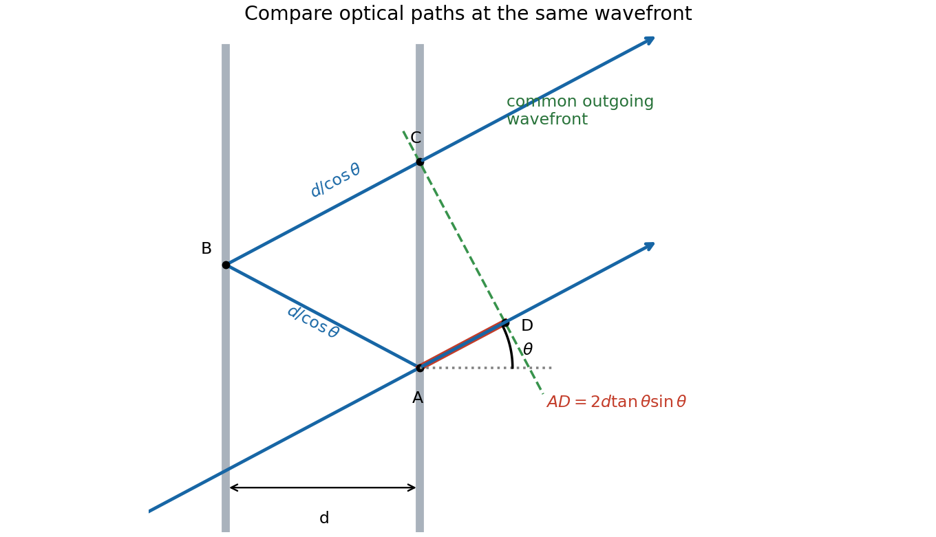
One extra round trip and the common outgoing wavefront in an air-spaced Fabry–Pérot interferometer
. Details. Count two electron spin states in each reciprocal-space cell of volume . Filling a Fermi sphere at zero temperature givesThe free electron model then givesThe energy zero is the bottom of the model's conduction band. The supplied carrier density already incorporates the one-electron-per-atom assumption; it must not be multiplied by another atomic count.
Write for the primitive cubic lattice spacing. With wavevector convention , reciprocal-lattice primitive vectors have length . The first Brillouin zone is the cube , henceIt has the same volume as any primitive reciprocal unit cell. A reciprocal coordinate defined in cycles per metre would instead give ; that is a different convention from this -space convention.
Take , and define and . Substitution of into the unforced equation gives . The roots determine whether the return is oscillatory.
For return after a displacement in this ideal model, critical damping, case (b), is the usual comfort choice: it removes repeated bouncing while avoiding the slow relaxation mode of strong overdamping. For release from rest it gives a monotone return with the fastest asymptotic decay available without oscillation. This criterion does not prove optimal comfort for every road profile or initial velocity; actual comfort also depends on acceleration, road forcing and suspension travel.
For the forced response, set and use . ThenThe general forced solution adds the appropriate homogeneous transient from (a), (b) or (c). Initial data were not specified, so its constants cannot be fixed. Positive damping removes this transient at long times. This solution uses the particular driving force in the supplied equation; it does not silently replace it by a different moving-support model.
Maximising is minimising its squared denominator . Differentiation givesA nonzero displacement resonance exists only if . Here , and thereforeThe low-frequency limit is , whereas at large . The parameters give damping ratio , consistent with an underdamped system and the existence of this amplitude maximum.
For , define . The two characteristic roots are real and negative:This is overdamping: there is no repeated oscillation, and the slow root controls late-time return. A generic initial velocity can still cause a single crossing of equilibrium, so “nonoscillatory” need not mean monotone for all initial data. For large , the slow root approaches .
For , the repeated characteristic root requires a second linearly independent solution :This is critical damping. If and , then , demonstrating the monotone return used in the suspension discussion.
For , put . Complex-conjugate roots give the real solutionThis is underdamping: oscillation at persists within a decaying exponential envelope. damping reduces the oscillation frequency below . Constants in all three cases are determined by two initial conditions.
For a monochromatic wave, a constant phase moves at phase velocity . For a narrow wave packet around , expansion shows that its envelope moves at group velocity . The envelope interpretation requires a sufficiently narrow spectrum and weak distortion; it is not a general identification with a causal signal front. Since and ,For the gravity-capillary wave, put and take . Direct differentiation givesThus when , orAt this wavelength the gravity and surface-tension restoring terms contribute equally. Also with positive second derivative: this is the minimum phase speed of a gravity-capillary wave, . Locally the carrier crests and narrow envelope travel together. The medium has not become nondispersive: there, so a finite wave packet can still spread. In the gravity-dominated limit ; in the capillary-dominated limit it tends to .
Take the aperture in and the observation point , with . Under scalar diffraction theory, the Huygens-Fresnel principle sums complex amplitudes from area elements, rather than summing their intensities. Apart from a common normalization,Here is the complex aperture transmission, is the axial distance, and is the angle of the secondary ray to the aperture normal. The obliquity factor describes the direction dependence of the secondary contribution; one Kirchhoff convention is for normal illumination. Other scalar boundary approximations have slightly different angular weights, all tending to unity near the axis.
Put . The paraxial approximation gives in the phase and in the amplitude. Removing common yieldsAssumptions are uniform normally incident plane-wave illumination, coherent monochromatic propagation, aperture dimensions large enough for the scalar description, , and phase accuracy over the relevant aperture. The last condition justifies dropping the quartic distance term; geometric smallness alone does not guarantee phase accuracy.
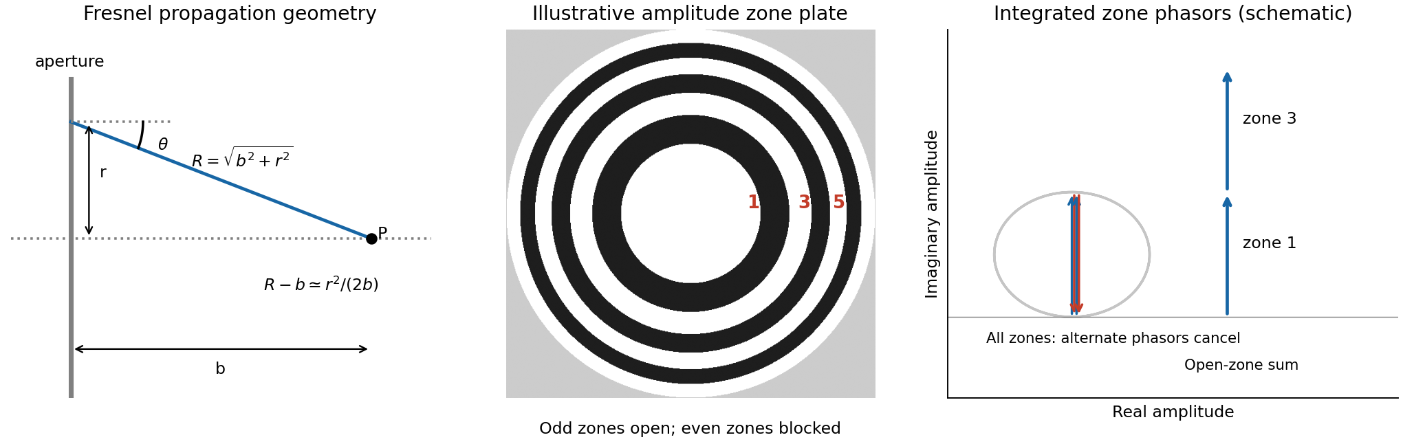
For a circular aperture, for and zero elsewhere. Rotational symmetry and give , , andThe constant can be absorbed into the proportionality factor, producing the required one-dimensional integral.
At a focus a distance away, half-period-zone boundaries obeyWith slowly varying obliquity and illumination, each zone has almost the same area and its integrated phasor has the opposite sign to its neighbour. A zone plate blocks alternate zones, so the remaining phasors add instead of nearly cancelling. Choosing an open central zone, the first three open regions have outer boundaries :These are outer radii, not zone widths; the second open region is the annulus between and .
For the specified outer radius, : there are approximately 49 half-period zones, of which 25 odd zones are open. Normalize to the field of the unobstructed plane wave. The normalized Fresnel aperture integral isFor any odd open annulus this gives , so the whole plate gives andThe axial intensity gain of an amplitude zone plate grows as the square of the number of open zones. Treating the number of zones continuously gives , the same accuracy as an estimate. This large local intensity gain is consistent with conservation of energy because light is concentrated into a small focal spot. It is not a power efficiency; the ideal first-order power efficiency of a binary amplitude zone plate is only .[ref]
Zone Plates by Janos Kirz and David Attwood. X-Ray Data Booklet, §4.4, first-order efficiency paragraph
“Without the zone plate” has here meant removing the finite plate and its outer stop, giving the unobstructed incident wave. If instead a clear circular aperture of radius is retained, its axial field is , so the ratio to that finite-aperture reference is . The two reference experiments differ; neither ratio should be confused with total transmitted power.
A Michelson interferometer divides a source beam at a partially reflecting beam splitter. The two perpendicular arms terminate in mirrors whose reflected beams return to the splitter and overlap at the detector. The recombined fields must have overlapping wavefronts and compatible polarization of waves. Moving one mirror by changes the round-trip optical path difference by , so passing fringes determine . Conversely a known mirror displacement measures wavelength. Scanning the delay can determine temporal optical coherence and, by Fourier transform spectroscopy, spectral structure. A compensating plate may equalize glass traversal, particularly for broadband illumination.
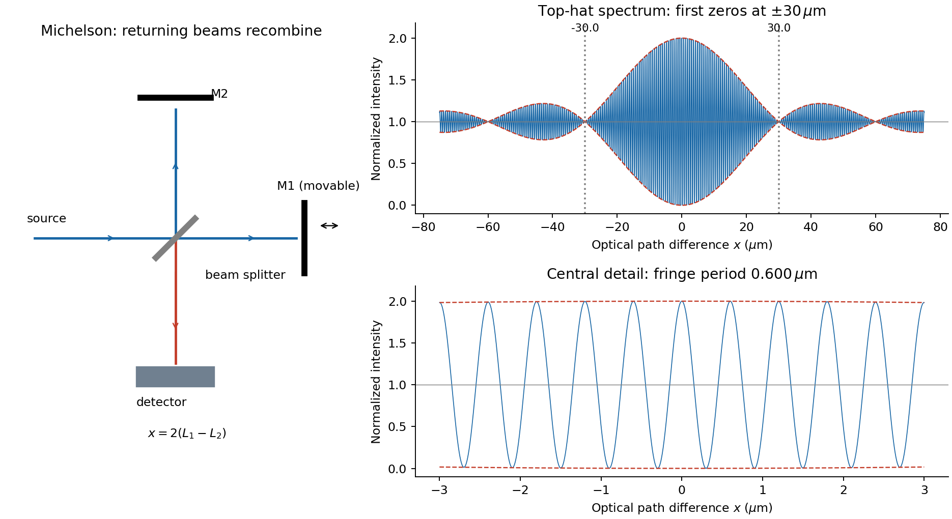
For equal real peak field amplitudes, the superposition isTime averaging the square over many optical cycles gives . With after absorbing a constant port-dependent phase into the zero of ,Here is the sum of the two separate-arm intensities; maximum intensity is and the ideal minimum is zero. Equal amplitudes give unit interference visibility.
For a stationary source with a flat intensity spectrum, different spectral components add in time-averaged intensity. Keeping their individual two-arm interference terms and defining givesOne must not coherently add unrelated source frequencies as if they had a fixed common phase. The sinc envelope is the Fourier transform of the rectangular spectral intensity.
Numerically, and . The annotated interferogram usesIt is even in , has central value 2 and background 1, and its carrier-fringe period in optical path difference is . The first envelope zeros are at , corresponding to mirror shifts of from equal paths. Side lobes persist beyond the zeros; a negative sinc reverses fringe phase. The intensity remains between and , not between the signed sinc curves with an assumed fixed ordering.
The free electron model replaces the microscopic ionic potential and interacting electronic motion by independent mobile electrons in a uniform neutralizing background, with approximately parabolic dispersion . Its quantum version fills states according to Fermi-Dirac statistics and the Pauli exclusion principle. Scattering is represented by a momentum relaxation time , rather than derived from the model's ideal free trajectories. This model explains a Fermi energy much larger than room-temperature thermal energy, an electronic heat capacity proportional to temperature at low temperature, and a Drude electrical conductivity. With appropriate scattering assumptions it also yields the Wiedemann-Franz law. It cannot by itself explain band gaps, detailed band anisotropy, strong correlations, or the microscopic temperature dependence of .
The inertial term is mass times the rate of change of mean drift velocity. The electric force is , taking the printed as the signed electron charge, and describes loss of directed momentum to scattering. electrons retain large microscopic velocities; this damping is of their mean directed motion. In a steady DC field,Both charge factors are negative for electrons, so the conductivity is positive. If instead denotes a positive charge magnitude, the force and current equations each require a minus sign and give the same result.
For AC response choose physical fields as real parts of phasors proportional to . Substitution givesThusThe real part decreases from to zero. The imaginary part starts at zero, reaches at , and falls as . The real part falls as at high frequency. With an convention, only the sign of the imaginary part changes. Positive gives positive cycle-averaged dissipation .
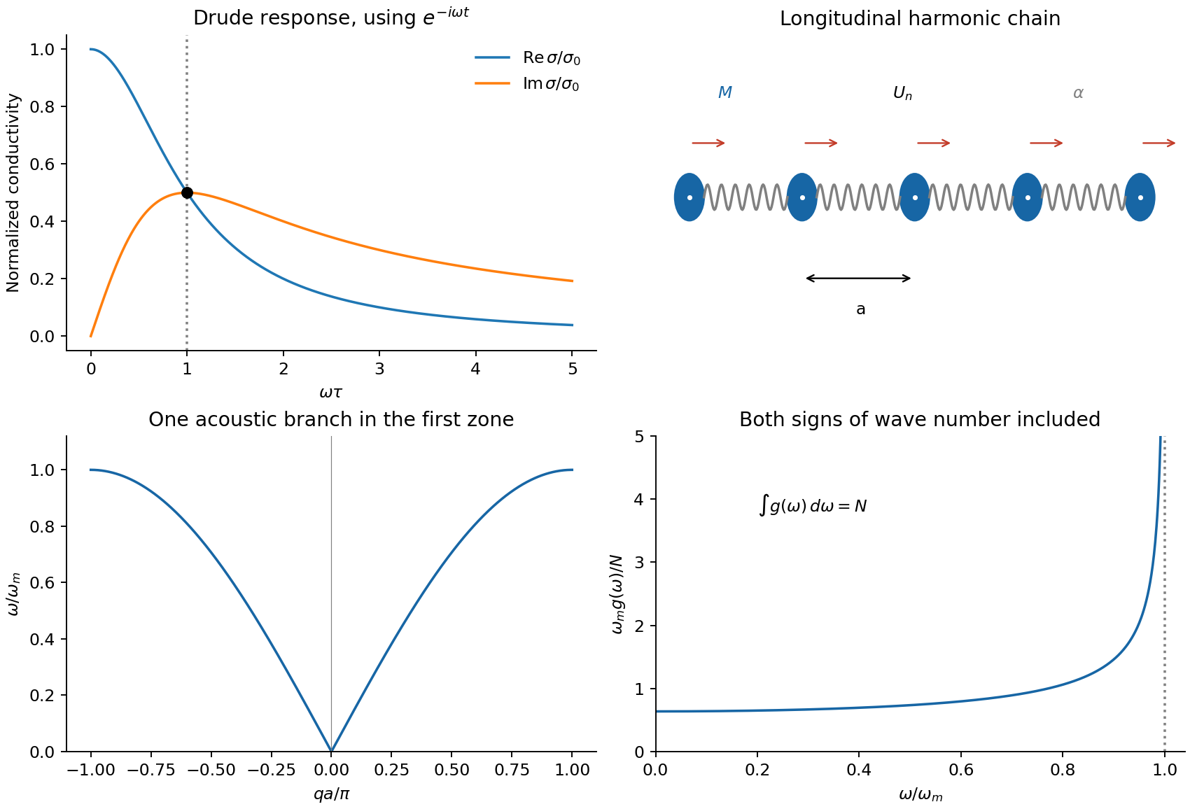
The supplied DC conductivity determines the transport time:Inertia matters when , giving , or . Quoting the former number as hertz would introduce an erroneous factor of .
Write the real displacement as , choosing real positive peak amplitude . Nearest-neighbour harmonic springs store energy in their extension , each spring counted once. Therefore the instantaneous physical energy isThe printed complex displacement is a calculation device: squaring the complex phasor itself would not produce physical energy. The chain sketch in the accompanying figure shows masses at equilibrium spacing , with longitudinal displacements along the chain.
The two spring forces on site giveSubstituting the normal-mode phasor and cancelling its nonzero amplitude givesThe long-wavelength limit is acoustic, , and the first Brillouin zone ends at . The maximum angular frequency is .
Time averaging uses . ConsequentlyThe dispersion relation makes these two contributions equal, givingThis is equality of time-averaged kinetic and potential energies in a harmonic normal mode; the instantaneous energy partition need not be equal.
Use periodic boundary conditions on length to count modes: . The density on the signed axis is . Using folded wave-number counting for a monatomic chain combines and at positive magnitude and counts both directions, so the convention used by the requested expression isThis is a large- continuum density, not a second independent branch. It gives modes after integrating over that half-zone; endpoint counting changes only finite-size corrections.
For positive , andThe density of states of a monatomic harmonic chain vanishes outside the band, is constant to leading order near zero, and has an integrable Van Hove singularity at the upper band edge where group velocity vanishes. Normalization checks the directional counting:
A completely filled valence band carries no net current: its occupied crystal-momentum states have velocities that cancel. Near a valence-band maximum, an almost full band is conveniently described by the few missing electrons, or electron holes. Removing an electron of charge , with , changes the charge relative to the filled band by . This is a quasiparticle description of electronic motion, not a mobile positive ion or a Positron.
For an isotropic parabolic maximum, . Assign the missing-electron state momentum and hole energyIt has positive effective mass . Its velocity equals the velocity of the missing electron state, and its positive-charge current replaces the negative of that state's electronic current. Semiclassical motion is thus . With momentum relaxation time , the low-field mobility is andIf electrons also contribute, : the two species' longitudinal conductivities add.
A Hall bar separates carrier concentration from mobility. Apply current density , magnetic field , and measure transverse electric field . For one isotropic hole population, transverse force balance gives , soFor thickness , the Hall-voltage magnitude is . A longitudinal four-terminal resistance measurement supplies independently. Use ohmic contacts, known conducting thickness, controlled temperature and low enough current to avoid self-heating. Reversing magnetic field removes even-in-field longitudinal offsets from contact misalignment; reversing current also helps reject thermoelectric offsets. These are central controls, rather than merely taking one transverse voltage reading.[ref]
Resistivity and Hall Measurements by National Institute of Standards and Technology. Sample Geometry; Resistivity Measurements; Definitions for Hall Measurements; Hall Measurements and Hall Calculations
The simple inference assumes one carrier type and a known Hall scattering factor. More generally , so measures Hall mobility rather than automatically the drift mobility. With two carrier populations at weak field,Its sign alone need not identify the more numerous carrier. A Hall experiment also cannot determine and separately: their ratio sets mobility. cyclotron resonance supplies an independent mass measurement by sweeping frequency or magnetic field through and detecting resonant absorption. The measured cyclotron effective mass can depend on band anisotropy and need not equal every curvature mass; the isotropic parabolic model identifies them. Its linewidth provides a scattering-time estimate only with a specified damping model.
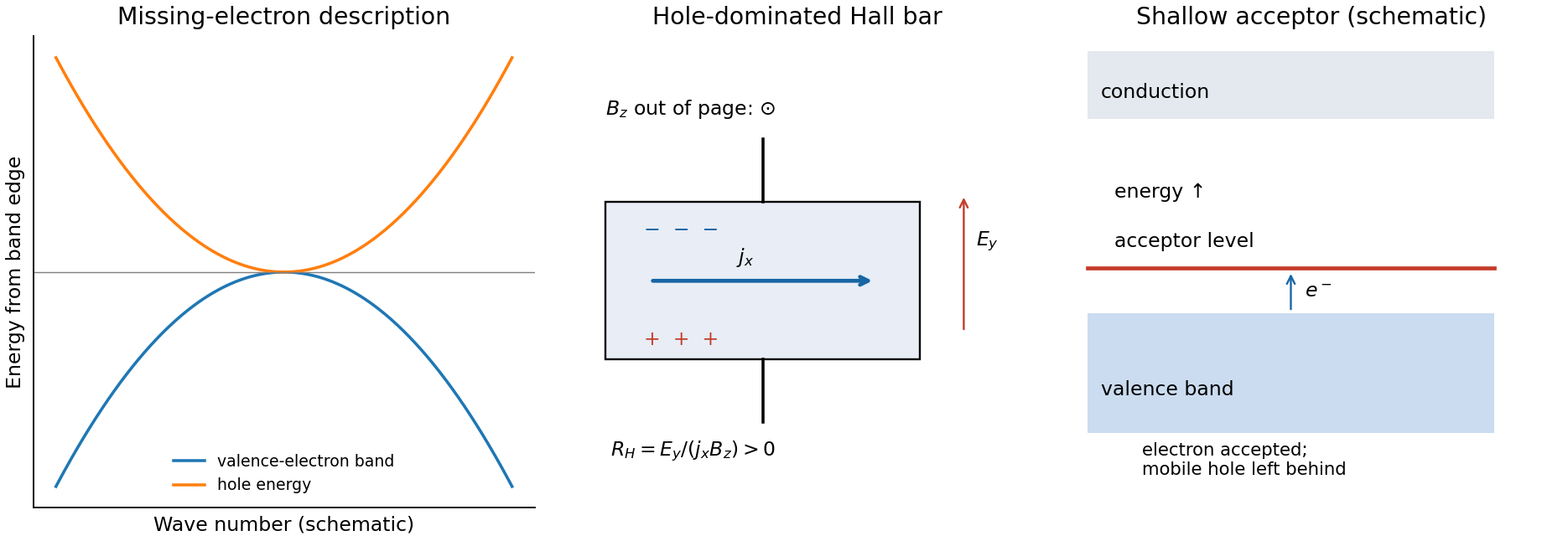
semiconductor doping generates holes by adding acceptor impurities. In silicon, a substitutional group-III atom such as boron provides one fewer valence electron than silicon. A shallow acceptor level lies slightly above the valence-band edge: accepting a valence electron makes the dopant negatively ionized and leaves a mobile hole in the valence band. The impurity stays fixed in the lattice. charge neutrality and the nondegenerate equilibrium mass-action law giveFor fully ionized, uncompensated acceptors in the extrinsic regime, and ; with fully ionized donor compensation, while holes remain dominant. The Fermi level moves towards the valence band. At low temperature, semiconductor carrier freeze-out suppresses mobile electron holes; at high temperature intrinsic electron-hole generation can dominate. Increasing dopant density also changes scattering, so a conductivity increase alone cannot distinguish increased carrier density from changed mobility. Temperature-dependent Hall and conductivity measurements separate these effects, subject to the carrier and scattering qualifications above.
For a small longitudinal disturbance, let the equilibrium pressure and mass density be , their perturbations be , and the fluid velocity be . Linearizing conservation of mass and the inviscid momentum equation in one dimension givesWhen compression is adiabatic, the equation of state gives with . Differentiating and eliminating yieldsfor an ideal gas with heat-capacity ratio and molar mass . Compression raises temperature as well as density, explaining the factor compared with the isothermal value .
A rightgoing plane sound wave has pressure and particle velocity in phase, , and mean intensity for peak amplitudes. Particle displacement is a quarter-cycle out of phase with particle velocity: particles oscillate locally while the compression pattern transports energy. This continuum linear description requires wavelength much larger than the mean free path, small pressure perturbations and negligible viscous attenuation. Adiabatic propagation requires heat exchange across the compressed region to be slow on the oscillation time; strong thermal coupling would instead favour an isothermal response.
The Q factor measures stored energy relative to loss: , or in the weak-loss limit. For viscous damping , write , and . The conventional oscillator parameter isIn free ringdown, fit the amplitude envelope . Its decay time is , whereas the cycle-averaged energy envelope decays on ; thus . Equivalently the logarithmic decrement between same-sign peaks is . It gives for weak damping, or the exact parameter relation . Fit multiple peaks above the noise floor, measure the damped period, and verify an exponential envelope rather than assuming all amplitude loss is viscous.
For a driven measurement, allow transients to settle and scan frequency at fixed force amplitude. Near resonance and at high , the response is Lorentzian in displacement power, with half-power points at displacement amplitudes of the maximum. Their angular-frequency separation gives . Halving the amplitude is not a half-power criterion.
The absorbed-power bandwidth of a viscously damped oscillator can be found exactly. Sinceits maximum is at , and the half-power frequencies satisfy . HenceFor broad resonances, displacement and absorbed-power peaks differ, so the measured observable must be specified. Frequency-dependent drive, backgrounds or several overlapping modes can otherwise masquerade as a changed Q factor.
For propagation along , a transverse wave has two perpendicular displacement components. With , write , . Their trajectory at a fixed point obeysThe general nondegenerate trajectory is an ellipse: elliptical polarization. For or , the components remain in phase or antiphase and the trajectory collapses to a line. A single nonzero component is also linearly polarized. Equal amplitudes with give circular polarization. Unequal quadrature amplitudes give an ellipse aligned with the chosen axes, while general phase differences rotate its axes.
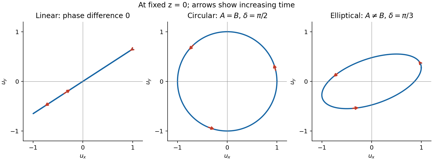


For the displayed convention and , at the vector starts at and moves towards as time increases. Reversing reverses its rotation. Right- and left-handed labels require a stated viewing and phase convention, so rotation is defined explicitly here. A fixed ellipse is a coherent relationship between transverse components; unpolarized light instead has fluctuating orientation and phase relationships on the measurement timescale.
A linear polarizer transmits a linearly polarized beam with intensity proportional to , allowing its direction to be measured by an analyser. circular polarization transmits equal intensity through any linear analyser, but that test alone does not distinguish it from unpolarized light. A quarter-wave plate converts a suitable coherent circular state to linear polarization, allowing the combination to discriminate them. For light the electric field defines the usual polarization; the magnetic field remains perpendicular to it and to propagation. Longitudinal sound in a homogeneous gas lacks the two transverse degrees of freedom needed for these polarization states.
Articles by others on the same topic
There are currently no matching articles.