Past exam of the physics A course of the University of Cambridge / 2018 / Paper 1 / Section D / D12

A chi-squared test compares residuals with the random scatter predicted by a model. For independent measurements $y_i$ with known Gaussian standard deviations ${\sigma }_i$ and predictions ${\mu }_i(\theta )$, formIf the mean model and error assumptions are correct, a full-rank linear fit of $p$ parameters gives a chi-squared distribution with $\nu =N-p$ statistical degrees of freedom. With a fully specified prediction and no fitted parameters, $\nu =N$. Nonlinear fits usually make this an approximation. Independent external calibration is not the same as fitting a parameter to these test data.

Under the reference distribution, the mean statistic is $\nu$ and its variance is $2\nu$. The upper-tail p-value $\mathrm{Pr}({\chi }_{\nu }^2\ge Q_{\mathrm{obs}})$ quantifies how unusual a discrepancy at least this large would be under the assumed model. A small value suggests model failure or incorrect uncertainties; it is not the probability that the model is true. An unusually small statistic can also reveal inflated uncertainties or correlations. A rejection threshold should be specified in advance.

For independent Poisson distribution counts, the model variance is its expected count ${\mu }_i$. The Pearson chi-squared statistic is $\sum (y_i-{\mu }_i{)}^2/{\mu }_i$. The estimated-error alternative ${\sigma }_i\simeq \sqrt{y_i}$ is common for large counts but can differ substantially when counts are small. In that regime the Poisson deviance or a direct likelihood calculation is preferable, with simulation if an accurately calibrated goodness-of-fit probability is required.

An exponential count rate appears as a straight line on a semilogarithmic plot:The early points decrease by roughly a factor $e$ per added sheet. Keeping the supplied $N_0$ fixed, a simple unweighted straight-line estimate from the first four logarithms isso the early trend is consistent with $b$ near one. This logarithmic estimate is illustrative; the final statistical comparison should use the count uncertainties rather than treating the logarithms as equally precise.

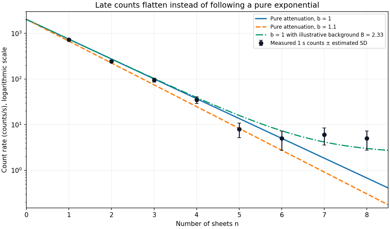
The pure exponential gives a useful approximate description through about the first four or five sheets. The first four observations are the clean high-count range; the fifth remains compatible with $b=1$ within its counting scatter. At $n=6,7,8$ the measurements are roughly constant at a few counts per second, so a single straight line no longer describes the whole pattern. Agreement of the sixth point with one exponential prediction by itself does not remove the systematic late flattening. There is no sharply determined physical cutoff from eight noisy measurements; the range used for a formal test should be stated explicitly.

Assume independent radioactive detections with negligible dead-time loss, so accumulated counts have a Poisson distribution. The reference measurement has total count $K_0=N_0{t}_0=2018500$ over $t_0=1000\mathrm{s}$. Since a Poisson count has variance equal to its mean, the rate uncertainty isIts relative uncertainty is $7.04\times 10^{-4}$, or $0.0704\%$. For each one-second measurement, ${\sigma }_y\simeq \sqrt{y}$, giving the estimated count and rate uncertaintiesin counts, numerically the same in counts per second for these one-second exposures. Their fractional uncertainties range from about $3.7\%$ at the first sheet to $35$–$45\%$ for the smallest counts. The long, high-rate reference is therefore much more precise. These are statistical errors; a longer exposure does not automatically remove calibration errors, source drift or background bias.

For a candidate attenuation coefficient, the one-second expected count is ${\mu }_n=2018.5e^{-bn}$. The model predictions areUse first the conservative signal-dominated range $n=1,\dots ,4$, where the count approximation is reliable and background is a small correction. Using the estimated errors from part (c), the weighted residual statistic isIt gives $\boxed{Q_{\mathrm{obs}}(1)=4.45,Q_{\mathrm{obs}}(1.1)=12.74}$. Since both $b$ candidates are fixed and $N_0$ was calibrated independently, neither was fitted to these four counts: the approximate reference has $\nu =4$, not three. The upper-tail probabilities are approximately $0.349$ and $0.0126$, respectively. Thus $b=1$ is compatible with the scatter, whereas $b=1.1$ is disfavored at the usual $5\%$ level in this approximate test.

A Pearson chi-squared statistic, using model variances instead of estimated observed variances, gives the same preference:Including the fifth point also leaves the decision unchanged: the estimated-error statistics are $8.37$ and $12.74$ on five degrees of freedom, with approximate upper-tail probabilities $0.137$ and $0.0259$; the Pearson statistics are $6.34$ and $15.63$. HenceThe small uncertainty in $N_0$ contributes correlated prediction uncertainty, as in chi-squared comparison of a calibrated attenuation model, but is negligible compared with the one-second counting errors here. Choosing the test range after inspecting the observations limits a strict interpretation of its nominal significance; the numerical comparison and its stated range are the relevant evidence.

If all eight observations are inserted into the estimated-error formula, the totals are $14.99$ and $22.48$. Their nominal eight-degree-of-freedom calibration is unreliable because the final expected counts are much smaller than one for some predictions. In fact the full-range Pearson statistics are $43.34$ and $118.25$, exposing the late excess much more strongly. The full Poisson deviance values are $24.09$ and $47.03$, again favoring $b=1$ but signaling that a background-free exponential is inadequate over the complete range. These sparse-count comparisons should not be used to claim that either unmodified model explains all eight measurements.

Introduce an additive background rate $B$, from ambient radiation, detector dark counts or another weakly attenuated contribution. If $S_0$ denotes the unattenuated signal alone, the attenuation count model with an additive background isIt approaches a nonzero constant as the transmitted signal becomes small. The source-off background should ideally be measured in a separate long exposure and its uncertainty included in the fit; otherwise estimate $B\ge 0$ jointly using a Poisson count likelihood.

There is a normalization detail: the given $N_0$ was itself obtained from an $n=0$ count measurement. If that measurement included the same background, then it measures $S_0+B$, and the attenuation fit normalized to a total reference rate isWriting $N_0{e}^{-bn}+B$ instead treats $N_0$ as a background-subtracted signal calibration. The difference is small here because the background is a few counts per second while $N_0$ is about two thousand, but the distinction prevents double-counting background. The last three observations alone do not give an exact value of $B$, because residual transmitted signal and sizeable counting fluctuations remain.