For a neutral atom, count both the nucleons and the electrons. Protons, neutrons and electrons are all fermions, and exchanging two identical intact atoms produces the sign from exchanging their fermionic constituents. An odd number gives a composite fermion; an even number gives a composite boson, consistently with the Spin-statistics theorem.
A lithium atom has three protons and three electrons. Lithium-6 also has three neutrons, giving fermionic constituents; lithium-7 has four neutrons, giving . ThereforeThe composite statistics of neutral atoms cannot be inferred from the mass number alone: counting only nucleons would classify the nuclei and give the opposite answers here. The atom's total spin includes its electrons as well as its nucleus.
The infinite square well has energy levels , with . The longest absorption wavelength corresponds to the smallest available energy difference from the ground state, namely . Its position matrix element is nonzero because the two states have opposite parity about the center of the well, so it is an allowed electric dipole transition.
Equating the photon energy to this gap givesHere the photon gap is approximately , not the ground-state energy itself.
In the orthonormal eigenbasis , the spin one-half operator is . An eigenvector with eigenvalue obeys and . A nonzero vector requires . Choosing normalized quantum phases givesThese spin eigenstates are orthogonal and have unit norm because and do.
Substitution in the moment of inertia givesFor independent errors interpreted as standard uncertainties, logarithmic differentiation and propagation of uncertainty giveConsequentlyThis is a statistical precision requirement. If “accuracy” instead means hard bounds whose worst cases must be guaranteed, first-order absolute errors add: , giving to first order. For an exact symmetric hard bound about the nominal values, the upper extreme is slightly more restrictive: gives , or . The question does not distinguish a statistical uncertainty from a worst-case tolerance, so the convention matters.
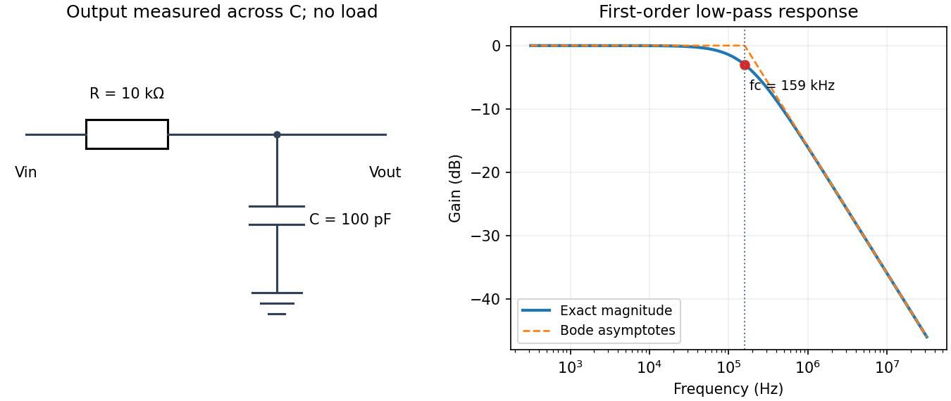
Use an unloaded RC low-pass filter: a series resistor between the source and the output node, with a capacitor from that node to ground, and measure the output across the capacitor. The components are ideal in this first-order model; “ideal” here does not mean a brick-wall frequency response.
The time constant is , henceThe capacitive electrical impedance gives the transfer function , soOn the magnitude Bode plot, . The gain approaches for , is at , and falls with slope per decade for . These results assume negligible source resistance beyond the specified and a sufficiently large load impedance.
Let be the probability density. For a real potential energy , the Schrödinger equation and its complex conjugate areDifferentiate and substitute both equations. The potential terms cancel, leavingComparison with the probability continuity equation identifiesFor a plane wave of amplitude and positive wavenumber , , the density times the velocity. Integrating the continuity equation over an interval makes its probability change equal to the incoming current minus the outgoing current.
SetAll are real and . Suppressing a common time quantum phase , chooseThe rightmost region has no left-moving term because no wave is incident from the right. The shifted quantum phase convention makes the transmitted amplitude at the second interface.
For finite potential steps and equal mass, wavefunction matching at a finite potential step requires continuity of both and . Explicitly,A discontinuous wavefunction would introduce an inadmissible singular kinetic term, while integrating the stationary Schrödinger equation across a finite step shows that the derivative cannot jump. These conditions also keep the probability current continuous, so a finite interface neither creates nor destroys probability. The derivative rule would need modification for a delta-function potential or a different effective mass; neither occurs here.
Zero reflection means . Matching the first interface then givesThe specified layer quantum phase is , so and . The second-interface conditions becomeSince , compatibility requires . This is a quantum quarter-wave matching layer: the intermediate wavenumber is the geometric mean, and the two interface reflections cancel after their round trip through the layer.
In terms of the physical energies,Rearranging also givesA finite positive energy satisfying the stated ordering requires . Under that condition , consistent with the assumed propagating transmitted wave. The width must simultaneously satisfy the given quarter-wave quantum phase condition.
From the second-edge amplitude in part (c),This uses . If the transmitted wave is instead written , its coefficient is ; the extra factor only changes the quantum phase convention.
Using the probability current of a plane wave,Thus the flux transmission probability is one. The larger transmitted density compensates for the smaller transmitted velocity ; equal currents need not have equal wave amplitudes.
The one-dimensional time-independent Schrödinger equation isHere is the particle mass, its potential energy, the stationary energy eigenvalue, and the reduced Planck constant. The spatial wavefunction is ; the full stationary state is . Physical bound states satisfy the boundary conditions and wavefunction normalization . The operator on the left is the Hamiltonian operator, the sum of kinetic and potential energies.
Assume and define so that the potential is that of a quantum harmonic oscillator. The two trial forms have derivativesSubstitution into the stationary Schrödinger equation cancels the terms precisely when . Normalizability selects the positive root,The remaining constants giveFor later overlaps choose positive normalization constants. The Gaussian integral gives , while its second-moment integral gives . Thus both wavefunctions have unit norm and are orthogonal by their opposite parity.
The real Gaussian is positive everywhere and has no nodes; the odd state has exactly one node at . The Sturm oscillation theorem orders one-dimensional bound states by their node count. Consequently these are the ground state and first excited state, respectively, also agreeing with the oscillator spectrum .
The infinite wall imposes , and the wavefunction vanishes for . The even full-oscillator ground state fails this boundary condition; the lowest admissible state is the positive-half restriction of the odd first excited state. Multiplying by restores normalization because half its probability originally lay on either side.
With , the half-harmonic oscillator ground state isIt rises from zero at the wall, reaches its wave-amplitude maximum at , and decays to zero as . It is positive throughout the interior of the allowed region, with no interior node, as required for its ground state. The wall need not make the derivative continuous with the forbidden half-line.
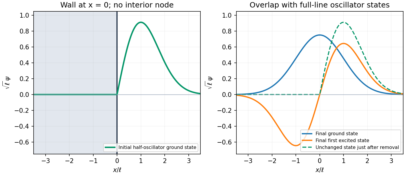
For removal of a half-oscillator wall, the sudden approximation keeps the state unchanged during the change of potential. Its probability in the new full-oscillator ground state is the squared overlap:where . ThereforeThe integral runs only over the initially occupied half-line. The initial state is not the odd full-line eigenstate: it is zero, rather than negative, on the left. Indeed its overlap with that final first excited state is , giving probability , and the remaining probability lies in higher states. Subsequent evolution under the new fixed Hamiltonian operator changes the quantum phases of its energy components without changing these energy-measurement probabilities.
The quantum rotor has orientation angle of period , so physical wavefunctions satisfy . The exponential solutions of are thereforeThey are normalized and orthogonal on . The corresponding angular momentum operator is , with eigenvalue . The ground level is nondegenerate, and every energy level has the twofold degeneracy . This uses ordinary periodic boundary conditions, with no flux or twisted quantum phase.
Expand the initial wavefunction in the angular momentum eigenbasis using . With the normalized from part (a), this givesThe coefficient squares sum to one, also verifying the stated normalization. The Born rule therefore gives angular momentum outcomesFor an energy measurement the two distinct states belong to the same energy eigenspace. Sum their probabilities, rather than adding their amplitudes, to obtainTheir relative probabilities are for the angular momenta and for the energies. In particular, zero mean angular momentum does not imply zero rotational energy.
Each energy eigenstate evolves by its own quantum phase . The two components have the same energy, while the quantum phase stays one. ThusIn angle representation this isAt , recovers the initial state. The fixed coefficient magnitudes keep the angular momentum and energy probabilities constant even though the density in angle changes.
Taking the modulus squared gives the three-mode revival of a planar quantum rotor:The angular density has period , while both the state and its density revive after . Its integral over is one because and .
At , the density is , with maxima at and zeros at . At it becomes , interchanging those maxima and zeros. At and , it is , with four equal maxima along the coordinate axes and positive minima halfway between them. At the original profile returns.
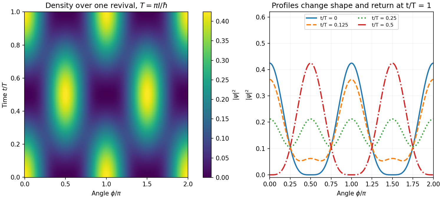
The changing profile is interference between the stationary mode and the degenerate counter-rotating modes. It does not translate rigidly around the circle; the standing-wave weights alternate between two orientations.
The commutator is . To evaluate it for differential operators, apply it to a smooth test wavefunction :Thus the canonical commutation relation is . The associated Heisenberg uncertainty relation is . Position and momentum cannot both have arbitrarily sharp outcome distributions in the same prepared state, even with ideal measuring apparatus. This concerns quantum-state preparation, not merely a calibration error in a particular instrument.
Expand the proposed product rule without interchanging any operator factors:Applying this commutator identity with and givesFor a differentiable multiplication potential, apply the other commutator to a test function:ThereforeThese operator equalities are understood on a common domain where the indicated products and derivatives are defined, with the boundary conditions appropriate to the state.
For a normalized state, the expectation value isFor a time-independent operator, differentiation givesThe Schrödinger equation says . The self-adjointness of gives , soIn the integral derivation, the same self-adjointness step is integration by parts with vanishing boundary terms. An explicitly time-dependent observable would also contribute . These are the expectation-value equations underlying the Heisenberg equation of motion.
The Hamiltonian operator isSince multiplication by commutes with multiplication by , part (b) gives . Similarly . Substituting into part (c) gives Ehrenfest theorem:Thus the mean momentum changes according to the mean force, and the derivative of mean position is mean velocity. These exact quantum equations resemble Hamilton's classical equations, but generally differs from . The classical point-particle equation for the center is exact for potentials at most quadratic and is an approximation for a localized packet when the force varies little across it. A spatially broad packet in a nonlinear potential need not follow a classical trajectory. Even where its center follows classical motion, its width and measurement uncertainties remain quantum properties.
The postulates of quantum mechanics give a framework for predicting observations from a prepared state. The experiments below motivate different features of that framework; no one experiment proves the whole set of postulates or specifies every Hamiltonian operator.
A pure quantum state is a normalized vector in a complex Hilbert space, with vectors differing by an overall quantum phase representing the same physical preparation. In position representation, . The linear state space permits quantum superposition, while the Born rule assigns probability to a position outcome in a region . The wavefunction is a probability amplitude; it is not a classical distribution of definite particle positions and momenta.
An observable is represented by a self-adjoint operator. If has spectral projectors , its possible measurement outcomes are its spectral values and . The mean is . For an ideal repeatable projective measurement, obtaining leaves the normalized conditional state . This projects onto an entire eigenspace if the outcome is degenerate. General detectors need more general measurement in quantum mechanics models; the projective update is an idealization. Noncommuting observables need not have simultaneous sharp values, as the canonical commutation relation and Heisenberg uncertainty relation illustrate.
Between measurements, an isolated system has unitary time evolution generated by its Hamiltonian operator:This preserves normalization and superpositions. Composite systems use a tensor product of state spaces, allowing entangled states as well as product states; identical particles additionally require the bosonic or fermionic exchange symmetry appropriate to their species. Statistical mixtures are described by a density matrix, with . These rules separate preparation, coherent evolution and measurement.
The photoelectric effect exposes discrete energy transfer by light. Illuminate a clean metal cathode in an evacuated tube and measure the collected Electron current while varying the light frequency, intensity and a retarding voltage. The stopping potential probes the largest emitted Electron kinetic energy, whereas the photocurrent measures the rate at which charge is collected. In the ordinary single-photon regime there is a threshold frequency; above it the maximum energy grows with frequency, rather than with intensity. Changing intensity at fixed frequency mainly changes the number of emitted electrons. These observations are summarized by the Einstein photoelectric equationHere is the surface work function, and the stopping voltage is understood after any photoelectric contact-potential correction. A photon delivers in an absorption event; emission is allowed only when that energy can pay the escape cost. This accounts for the frequency threshold and the lack of the classical waiting time associated with slowly accumulating energy in a single Electron. The experiment supports energy quantization of light; it does not imply that every incident photon emits an Electron or that every emitted Electron has the maximum energy. Surface losses and collection geometry affect the full current-voltage curve.
The Davisson–Germer experiment demonstrates a complementary wave property of matter. An Electron gun uses a heated emitter, accelerating voltage and apertures to send a narrow beam onto a nickel single crystal in vacuum. A movable collector measures scattered electric current versus direction; rotating the crystal also tests its azimuthal symmetry. The crystal gives sharp angular beams whose positions depend on voltage and crystal orientation. A prominent feature occurs near accelerating voltage and roughly detector colatitude. The nonrelativistic de Broglie wavelength predicted at that voltage isDiffraction wavelengths inferred using the known crystal structure agree with this voltage dependence. These angular peaks arise from coherent addition of scattering amplitudes from the crystal, not from classical specular reflection of independent point projectiles. Bragg's law is for lattice-plane spacing and angle to those planes; a detector colatitude is a different angle and must not be substituted without its geometry. The historical readout was current, not a photograph of individual Electron trajectories.[ref]
Diffraction of Electrons by a Crystal of Nickel by C. Davisson and L. H. Germer. 1927, apparatus pp. 707–710 and angular/voltage scans pp. 715–719
The double-slit experiment makes the role of amplitudes especially direct. A coherent source illuminates two narrow slits; an observation screen a distance away records the pattern. For slit spacing and small screen displacement , the path difference is approximately . The two amplitudes add before probabilities are formed:For equal coherent illumination the interference term varies as , giving fringe spacing beneath the single-slit diffraction envelope. Blocking one slit removes that cross term. Young's optical experiment established wave interference; later particle-resolved realizations with photons or electrons show localized detection events whose accumulated distribution has the interference pattern. Low arrival rates demonstrate that this pattern does not require different incident particles to collide with one another.
If the paths become correlated with distinguishable detector states and , the cross term acquires their overlap . Perfectly distinguishable path records make that overlap zero, suppressing interference even if the spatial beams still overlap. This connects quantum entanglement, measurement and loss of observable coherence. Without a path measurement, the two alternatives are amplitudes for one preparation, rather than classical mutually exclusive events whose probabilities may simply be added.
Together these experiments motivate a description in which energy transfer and detector outcomes can be discrete, yet propagation retains complex quantum phases and interference. The Born rule connects those amplitudes to repeatable frequencies of outcomes. The Schrödinger equation supplies the dynamics once a Hamiltonian operator is specified, while observable operators, state preparation and the measurement model specify what the apparatus can read.
Indistinguishable particles have the same intrinsic properties and cannot be assigned physically observable permanent labels. Exchanging their mathematical coordinates leaves all physical predictions unchanged. In ordinary three-dimensional quantum mechanics the total state, including spin, obeysThe Spin-statistics theorem associates integer spin with bosons and half-integer spin with fermions. Exchange does not mean physically transporting two particles along some prescribed trajectories; it is the symmetry of the many-particle state under permutation of its arguments.
For orthonormal one-particle states , normalized two-particle spatial combinations are . They illustrate coherent exchange amplitudes. If both fermions have the same complete one-particle state, the antisymmetric combination vanishes. This is the Pauli exclusion principle: a fermionic mode has occupation zero or one. Bosonic modes can have arbitrarily large occupation. A many-fermion product basis is antisymmetrized by a Slater determinant.
It is the full spin-spatial state that must have the appropriate symmetry. For two electrons, an antisymmetric spin singlet state can accompany a symmetric spatial orbital, so opposite-spin electrons can occupy the same spatial orbital. A symmetric spin triplet instead needs an antisymmetric spatial state. Thus exclusion concerns identical complete states, not an unconditional prohibition on sharing a position or spatial orbital.
Counting allowed occupations gives Bose-Einstein statistics and Fermi-Dirac statistics. For an ideal gas in thermal equilibrium,Bosonic accumulation permits Bose-Einstein condensation; exclusion gives a filled Fermi sea and degeneracy pressure even at zero temperature. In the dilute classical limit the occupations are small and both expressions approach the Maxwell-Boltzmann distribution. Exchange effects become important when wavepackets overlap appreciably, often characterized by number density times the cube of the thermal wavelength.
Composite particles follow their total exchange statistics while remaining intact. The composite statistics of neutral atoms depend on electrons as well as nucleons, as in the two lithium isotopes above. Symmetrization can produce bunching or antibunching in joint detection probabilities even in the absence of an interaction potential; it is not an additional classical force.
A diatomic molecule has one internal bond-stretching vibrational coordinate. Near its equilibrium separation, approximate the bond by a spring of stiffness and use the reduced mass . Its frequency is and its quantum harmonic oscillator levels are .
For independent molecules in thermal equilibrium, set . The single-molecule canonical partition function is a geometric series:Using , where , givesPer mole replace by . The zero-point energy is present in but is temperature-independent and contributes nothing to the heat capacity.
For , occupation of the first excited vibrational state is exponentially suppressed: . The vibrational degree of freedom is frozen out. For , . This recovers classical equipartition: the quadratic kinetic term and quadratic elastic term each contribute per molecule.
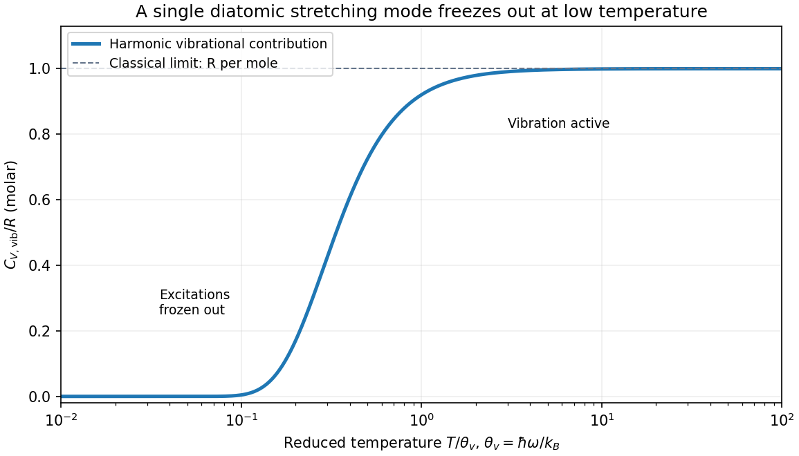
The vibrational heat capacity of a diatomic gas must be distinguished from the total heat capacity. In a dilute gas with rotations already active and vibration still frozen, translation contributes and rotation , so molar . Once vibration is active it adds , giving . For an ideal gas of a fixed number of intact molecules, , so the corresponding values are and . Very low temperatures also freeze rotations, while sufficiently high temperatures bring anharmonicity, dissociation or electronic excitations; the harmonic plateau is restricted to the range where those effects are negligible.
Quantum tunnelling is transmission through a finite classically forbidden region, where . The stationary Schrödinger equation permits an evanescent wavefunction inside such a barrier rather than forcing it to vanish at its entrance. Matching to propagating states beyond a barrier of finite width gives a nonzero transmitted probability current.
For a rectangular barrier of height and width , with equal exterior potentials and , write . The exact rectangular-barrier tunnelling probability isFor an opaque barrier its dominant dependence is . For a slowly varying barrier, the WKB approximation generalizes this to , apart from matching prefactors. Barrier width, particle mass and energy therefore have a strong influence. Energy is conserved in a static barrier: tunnelling does not require the particle to borrow energy or acquire a classical path with negative kinetic energy.
In alpha decay, a nuclear alpha-particle configuration is confined by the short-range nuclear interaction but separated from the exterior by a Coulomb barrier. Its energy can be positive relative to infinity while still lying below the barrier maximum. Escape by tunnelling produces alpha particles at that conserved energy, with an exponentially small decay probability per nuclear encounter. The pronounced dependence of half-life on alpha energy is a characteristic consequence of the barrier exponent, unlike a simple classical escape threshold.
In scanning tunneling microscopy, a conducting tip is brought within a nanometer-scale vacuum gap of a conducting surface and biased weakly. Electron tunnelling gives a current that depends approximately exponentially on separation, in a simple low-bias model. Feedback adjusts the tip height to keep current fixed while scanning, producing a surface map sensitive to both geometry and electronic states. Finite current through the non-contact gap, and its steep dependence on separation, are the direct tunnelling signatures; current is not a direct measurement of topographic height alone.
A Josephson junction provides a collective superconducting example. Two superconductors separated by a thin barrier can carry a coherent pair current even at zero voltage. At constant voltage the AC Josephson effect gives and oscillation frequency . The coupled condensate quantum phases and pair transfer distinguish this from independent normal-electron transmission. These examples involve different microscopic barriers, but all require quantum coupling across a region that suppresses classical passage. Comparing weak-temperature tunnelling behavior with thermally activated escape helps distinguish the mechanisms experimentally.
A chi-squared test compares residuals with the random scatter predicted by a model. For independent measurements with known Gaussian standard deviations and predictions , formIf the mean model and error assumptions are correct, a full-rank linear fit of parameters gives a chi-squared distribution with statistical degrees of freedom. With a fully specified prediction and no fitted parameters, . Nonlinear fits usually make this an approximation. Independent external calibration is not the same as fitting a parameter to these test data.
Under the reference distribution, the mean statistic is and its variance is . The upper-tail p-value quantifies how unusual a discrepancy at least this large would be under the assumed model. A small value suggests model failure or incorrect uncertainties; it is not the probability that the model is true. An unusually small statistic can also reveal inflated uncertainties or correlations. A rejection threshold should be specified in advance.
For independent Poisson distribution counts, the model variance is its expected count . The Pearson chi-squared statistic is . The estimated-error alternative is common for large counts but can differ substantially when counts are small. In that regime the Poisson deviance or a direct likelihood calculation is preferable, with simulation if an accurately calibrated goodness-of-fit probability is required.
An exponential count rate appears as a straight line on a semilogarithmic plot:The early points decrease by roughly a factor per added sheet. Keeping the supplied fixed, a simple unweighted straight-line estimate from the first four logarithms isso the early trend is consistent with near one. This logarithmic estimate is illustrative; the final statistical comparison should use the count uncertainties rather than treating the logarithms as equally precise.
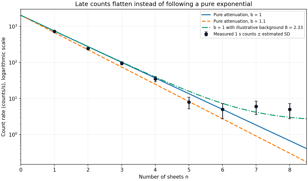
The pure exponential gives a useful approximate description through about the first four or five sheets. The first four observations are the clean high-count range; the fifth remains compatible with within its counting scatter. At the measurements are roughly constant at a few counts per second, so a single straight line no longer describes the whole pattern. Agreement of the sixth point with one exponential prediction by itself does not remove the systematic late flattening. There is no sharply determined physical cutoff from eight noisy measurements; the range used for a formal test should be stated explicitly.
Assume independent radioactive detections with negligible dead-time loss, so accumulated counts have a Poisson distribution. The reference measurement has total count over . Since a Poisson count has variance equal to its mean, the rate uncertainty isIts relative uncertainty is , or . For each one-second measurement, , giving the estimated count and rate uncertaintiesin counts, numerically the same in counts per second for these one-second exposures. Their fractional uncertainties range from about at the first sheet to – for the smallest counts. The long, high-rate reference is therefore much more precise. These are statistical errors; a longer exposure does not automatically remove calibration errors, source drift or background bias.
For a candidate attenuation coefficient, the one-second expected count is . The model predictions areUse first the conservative signal-dominated range , where the count approximation is reliable and background is a small correction. Using the estimated errors from part (c), the weighted residual statistic isIt gives . Since both candidates are fixed and was calibrated independently, neither was fitted to these four counts: the approximate reference has , not three. The upper-tail probabilities are approximately and , respectively. Thus is compatible with the scatter, whereas is disfavored at the usual level in this approximate test.
A Pearson chi-squared statistic, using model variances instead of estimated observed variances, gives the same preference:Including the fifth point also leaves the decision unchanged: the estimated-error statistics are and on five degrees of freedom, with approximate upper-tail probabilities and ; the Pearson statistics are and . HenceThe small uncertainty in contributes correlated prediction uncertainty, as in chi-squared comparison of a calibrated attenuation model, but is negligible compared with the one-second counting errors here. Choosing the test range after inspecting the observations limits a strict interpretation of its nominal significance; the numerical comparison and its stated range are the relevant evidence.
If all eight observations are inserted into the estimated-error formula, the totals are and . Their nominal eight-degree-of-freedom calibration is unreliable because the final expected counts are much smaller than one for some predictions. In fact the full-range Pearson statistics are and , exposing the late excess much more strongly. The full Poisson deviance values are and , again favoring but signaling that a background-free exponential is inadequate over the complete range. These sparse-count comparisons should not be used to claim that either unmodified model explains all eight measurements.
Introduce an additive background rate , from ambient radiation, detector dark counts or another weakly attenuated contribution. If denotes the unattenuated signal alone, the attenuation count model with an additive background isIt approaches a nonzero constant as the transmitted signal becomes small. The source-off background should ideally be measured in a separate long exposure and its uncertainty included in the fit; otherwise estimate jointly using a Poisson count likelihood.
There is a normalization detail: the given was itself obtained from an count measurement. If that measurement included the same background, then it measures , and the attenuation fit normalized to a total reference rate isWriting instead treats as a background-subtracted signal calibration. The difference is small here because the background is a few counts per second while is about two thousand, but the distinction prevents double-counting background. The last three observations alone do not give an exact value of , because residual transmitted signal and sizeable counting fluctuations remain.
Bayes' theorem updates prior knowledge using the likelihood of new observations. For alternative hypotheses ,The prior describes information before the data ; is the sampling likelihood, and the posterior describes the updated probabilities. Posterior odds equal prior odds times the likelihood ratio. A likelihood is a probability model for data at specified parameters, not automatically a normalized probability distribution over those parameters.
For a continuous parameter , the same rule uses densities: . Priors can encode positivity, physical limits, previous independent measurements or calibration knowledge. Their parameterization matters: a density uniform in a rate is not uniform in its logarithm. Proper priors make model evidences well defined; an arbitrary normalization in an improper prior is especially problematic for comparing models.
A counting example uses Poisson-gamma conjugacy. If a detector registers events in exposure with constant rate , . A gamma prior with shape and rate parameter , , givesThe posterior mean combines the prior rate with the observed rate , weighted by the prior and actual exposures. The parameters must use a consistent shape-rate convention. Small counts can leave substantial prior sensitivity; abundant informative data usually reduce it for regular identifiable models.
Independent old data can become the prior for a new experiment, giving the same result as joint updating under a consistent model. The new data must not also have been used to construct that prior, or the evidence is counted twice. A credible interval has a specified posterior probability under the chosen model and prior; this interpretation differs from repeated-sampling coverage of a confidence interval. Predictions for a future observation average its sampling distribution over the posterior, incorporating parameter uncertainty. Prior sensitivity checks and a defensible likelihood are therefore part of the inference, rather than Bayes' theorem itself supplying missing physical knowledge.
A systematic error is a reproducible bias in the measurement model or procedure, such as a zero offset, incorrect gain, background contamination, misalignment, loading or temperature-dependent calibration. Repeating the same biased procedure more often reduces independent random scatter but does not remove the bias. An unknown correction also has a measurement uncertainty, even when the mechanism is systematic.
A simple instrument model is , with gain error , offset , drift and random noise . Comparison with calibrated standards at several input values separates an offset from a scale error and can test nonlinearity. Use standards that cover the operating range, verify units and reference values, and propagate uncertainty in the standards into the corrected result. Calibration changes the model; it does not make the corrected measurement exact.
A blank or source-off measurement estimates additive background. For independent source-plus-background count in time and background count in time , the net-rate estimate and its counting variance areSubtracting a measured background removes its estimated mean, not its fluctuations or its uncertainty. A long background exposure can reduce the latter, while drifting backgrounds require monitoring or a joint model.
Reversal can distinguish a wanted signal from an unchanged offset. For example, and give when the thermoelectric offset is stable between readings. Interchanging sample and reference, reversing field direction or reversing an apparatus orientation can similarly expose sign-dependent biases, but only if the wanted and unwanted contributions transform differently.
Track slow instrumental drift using frequent references, interleaved readings or an ABBA measurement sequence. Equal-time readings in the order A, B, B, A cancel a common linear drift in the difference estimator . Nonlinear drift or unequal sample conditions can survive. Randomizing run order helps prevent a time drift from imitating dependence on a controlled experimental variable.
Control physical couplings directly: stabilize temperature, minimize gradients, shield unwanted fields, align geometry, and use high input impedance when loading is the concern. Differential and bridge measurements suppress common changes when their channels are well matched. Varying an apparatus parameter or using an independent method can reveal an unsuspected bias. Report residual corrections, their uncertainties and correlations; adding more identical readings cannot justify discarding a shared calibration uncertainty.
Johnson-Nyquist noise is equilibrium electrical fluctuation caused by thermal agitation of charge carriers. A resistor can generate a fluctuating terminal voltage even when its mean current is zero. In the classical frequency range , the Fluctuation-dissipation theorem relates this noise to dissipative resistance. The one-sided voltage power spectral density of an unloaded resistor isEquivalently its short-circuit current spectrum is . Over a flat bandwidth the rms voltage is . A real measurement instead integrates over positive frequency, with loading and the filter's effective noise bandwidth included. A flat spectrum does not imply an infinite physically measurable variance; the circuit and the quantum high-frequency regime limit the ideal white-noise model.
Cooling or narrowing the accepted bandwidth reduces thermal noise. Reducing resistance lowers its open-circuit voltage noise but raises its short-circuit current noise, so the appropriate choice depends on source impedance and amplifier loading. Thermal agitation is not a fluctuating externally applied voltage that can be removed by perfect shielding alone.
Shot noise arises from discrete transfer events. In the simplest shot noise counting model, equal charges arrive independently at constant rate . A gate of duration contains a Poisson number , with mean and variance . Therefore mean current is , and the averaged-current variance is . The corresponding one-sided low-frequency spectrum isfor a flat accepted bandwidth. Electron current has . Vacuum emission or photodetection can approximate independent arrivals; correlations in a conductor can suppress or enhance the fluctuations. Discreteness by itself does not guarantee Poisson statistics.
For a fixed mean current the ideal shot-noise formula is not proportional to temperature, whereas Johnson noise is. Increasing current raises absolute shot noise but lowers its fractional size, since . Both can appear approximately white within a useful frequency band, and independent noise powers add after referring them to a common measurement point. Their spectra must use the same convention: two-sided densities are half these one-sided values. A real low-current experiment can also contain amplifier noise, low-frequency drift and correlated transfer noise, so a mean current or resistance alone does not specify its complete noise budget.
For a photon, . Using Planck constant , speed of light and givesThe Rayleigh criterion for a circular aperture of diameter is , set by the first zero of its Airy disk. Thus the ideal diffraction-limited resolution isThe conversion to transverse separation uses the small-angle approximation. An order-of-magnitude estimate instead gives and ; the distinction is the chosen resolution criterion. These are aperture limits, before instrumental aberrations and detector sampling.
Both the incoming and outgoing spherical wavefronts contribute to the path excess. At aperture radius , with axial distances before and after the aperture,The outer edge of the th Fresnel half-period zone has . HenceTherefore the outer radius is . The paraxial approximation is excellent because . Treating the illumination as a plane wave would incorrectly omit the source-side path curvature.
At normal incidence between lossless media with real positive acoustic impedances , continuity of pressure and normal particle velocity gives the pressure transmission amplitude . Since the mean acoustic intensity is , the fraction of incident energy transmitted isThis is acoustic reflection and transmission at an interface. With the supplied acoustic impedances,A thin water-based gel layer excludes air gaps and approximately matches the body's acoustic impedance. About of incident energy would otherwise reflect at the air-body interface. The coupling is also needed on the return journey, so it strongly improves the detectable echo. These figures concern interface transmission, before absorption within tissue; the gel is approximated by the stated water value.
Take nearest-neighbour separation , a common spring constant , and one scalar displacement per atom. For a monatomic chain, the harmonic approximation near a potential minimum, Newton's second law and a normal mode giveThe monatomic-chain dispersion relation has one acoustic phonon branch, with near the origin. The first Brillouin zone ends at , where and the group velocity vanishes.
For alternating masses , choose a two-atom cell of length . The coupled normal modes give the diatomic-chain dispersion relation with equal springs,The first Brillouin zone now ends at . The minus branch is the acoustic phonon branch; its two atoms move together at long wavelength. The plus branch is the optical phonon branch; at the atoms move oppositely with a stationary centre of mass and . For the edge frequencies are and , with a gap between them.
If , the two branches reduce to and , touching at . This is zone folding in an equal-mass diatomic chain: identical sites actually have a primitive unit cell of length . A doubled cell folds the monatomic branch but opens no gap. Equal masses alone do not specify all possible spring models; the sketches assume equal nearest-neighbour spring constants.
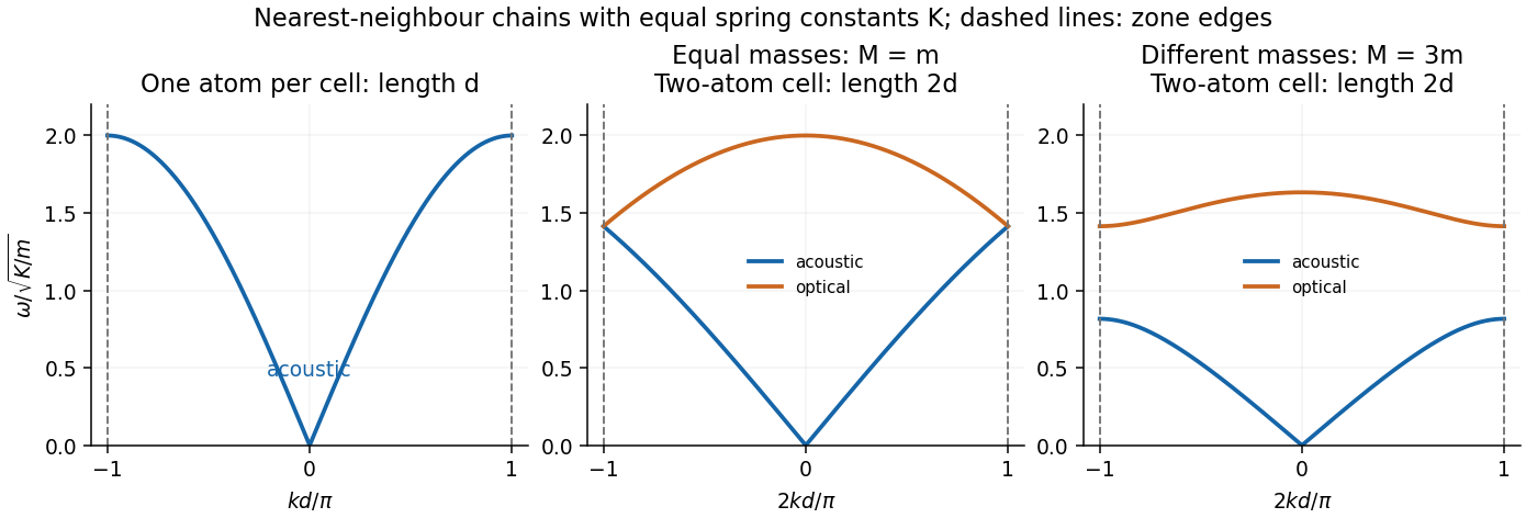
Monatomic and two-atom-chain dispersion relations, with explicitly chosen cell lengths and zone edges
. Details. Under the one-carrier Drude model, the magnitude of the Hall coefficient gives an effective carrier densityConvert the material mass density to and its molar mass to . The atomic number density isHere is the Avogadro constant. The positive Hall coefficient gives a hole-like response in a one-carrier interpretation. The Hall carrier count versus valence distinction matters: beryllium has two valence electrons, but the result is neither two free Electrons nor a literal fractional atom donating charge. Its energy bands and Fermi surface invalidate the simple isotropic one-carrier inference. Electron-like and hole-like contributions with different charge carrier mobilities can yield this sign and effective count.
Substituting into the damped harmonic oscillator equation givesFor nonnegative viscous damping, the cases areThe PDF's request to express these conditions in terms of is dimensionally inconsistent with its definition : already has units . With the unnormalised equation , the equivalent comparisons are , or . Also is the undamped natural angular frequency, not in general the driven displacement peak.
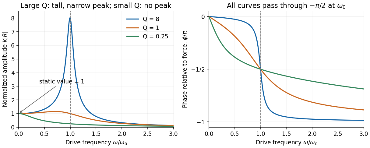
For the steady response of a forced harmonic oscillator, write and use the same complex amplitude convention for the driving force. Substitution givesThus the response magnitude and displacement phase relative to the force areThe phase goes from at low frequency, through at , towards at high frequency. The static magnitude is , while the high-frequency magnitude is approximately .
Define the quality factor by . If , the displacement peak occurs at ; for the magnitude decreases monotonically from its static value. For there is a tall narrow peak close to , of height approximately and width approximately . At very small the resonant peak disappears and the response is broad. The plotted functions are normalized as , at fixed .


The original diagram is a series RLC circuit, so the same electric current passes through all three elements. Choose capacitor electric charge positive on the plate into which positive enters. Kirchhoff's voltage law givesDividing by inductance givesThe correspondence to the forced harmonic oscillator is , , , and . The stored energy is ; its balance is , confirming the damping sign.
The capacitor-charge complex amplitude isFor fixed driving-voltage amplitude, maximizing minimizesDifferentiate:The positive-frequency minimum therefore hasThis is the resonance of charge, or capacitor voltage. If the stated inequality fails, their maximum is at zero frequency, and no positive displacement-resonance peak exists. The electric current has the additional factor , and instead peaks exactly at for every .
Articles were limited to the first 100 out of 171 total.
Articles by others on the same topic
There are currently no matching articles.