Past exam of the physics A course of the University of Cambridge / 2019 / Paper 1 / Section D / D12

An ideal operational amplifier has infinite differential open-loop gain, infinite input impedance, zero output impedance, unlimited bandwidth and slew rate, and zero input offset voltage, input bias current and intrinsic noise. The idealized model has no finite output-swing or output-current limit.

The usual circuit rules areThe first follows from infinite input impedance. The second follows because a finite output requires $v_{+}-v_{-}=v_o/A\to 0$ as the open-loop gain tends to infinity. It is a virtual equality of potentials, not a conducting connection between the inputs. It cannot be imposed for open-loop operation or after an amplifier reaches its supply rails.

Let $v$ be the inverting-input potential. The non-inverting input is grounded, so the ideal operational amplifier rules give $v=0$ and no input current. Kirchhoff's current law at that node therefore givesIntegrating from an initial time $t_0$,This op amp integrator performs inverted time integration; the initial voltage across the capacitor supplies the integration constant. For zero initial conditions its transfer function is $H(s)=-1/(sRC)$. In sinusoidal steady state, with the convention $e^{i\omega t}$,For example, a cosine input produces a negative sine output after its constant component is set. The additional inversion makes the phase $+90^{\circ }$ modulo $360^{\circ }$, rather than the $-90^{\circ }$ of non-inverting integration.

Any direct-current component of the input produces an output ramp. The input offset voltage and input bias currents of a real operational amplifier therefore charge the feedback capacitor until the output saturates. Even the desired signal can exceed the available output swing when integrated for too long. Initial capacitor charge also introduces an unknown integration constant.

Place a large resistor $R_f$ in parallel with the feedback capacitor. The idealized transfer function then becomesIts finite direct-current gain $-R_f/R$ supplies a return path and bounds the response to a small offset; it approximates $-1/(sRC)$ when $\omega R_{f}C\gg 1$. The chosen gain must still keep offsets within the output range. A reset switch across the capacitor can set the initial charge, while low-offset amplifiers, bias compensation and input offset adjustment reduce drift. Useful integration also requires frequencies below the amplifier's own response limit.

A real operational amplifier has large but finite, frequency-dependent open-loop gain; the gain falls and its phase changes at higher frequencies. Finite bandwidth and slew rate constrain small-signal and large-signal responses respectively. There are also finite input impedance and output impedance, nonzero input bias currents and input offset voltage, and internally generated noise. Offset and bias can drift with temperature.

The output is limited by the supply voltages and output-current capability, and the inputs have a permitted common-mode range. Rejection of common-mode and supply changes is finite. Consequently $v_{+}-v_{-}$ need not vanish exactly, and neither the virtual-ground approximation nor linear gain formulas apply after saturation. For the calculation below the stipulated infinite input impedance removes the input loading currents, while finite gain and optionally finite output resistance are retained.

A non-ideal amplifier is not specified by infinite input impedance alone: its open-loop gain and output impedance must also be modeled. Take its internal controlled output to be $u=-A(s)v$, where $v$ is the inverting-input potential, and place a resistance $r_o$ between $u$ and the actual output $y=V_{\mathrm{out}}$. The non-inverting input remains grounded; assume no external load. This gives an explicit finite-gain operational-amplifier integrator model.

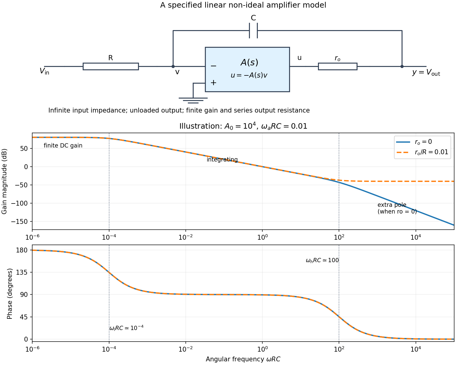
Writing Kirchhoff's current law at the input and output nodes givesThe second equation gives $y=(sC{r}_o-A)v/(1+sC{r}_o)$. Substitution in the first gives the general transfer functionFor sinusoidal phasors, set $s=i\omega$. The numerator and denominator are complex, so the magnitude gives the amplitude ratio and their arguments give the relative phase.

The simplest model takes $r_o=0$ and a constant finite gain $A_0>0$. It givesThus below ${\omega }_l=[(1+A_0)RC{]}^{-1}$ the amplifier has gain magnitude $A_0$ and inversion. Above that frequency it approaches an integrator with magnitude $A_0/[(1+A_0)\omega RC]\simeq 1/(\omega RC)$ and phase $+90^{\circ }$. Constant finite gain by itself predicts no further high-frequency turnover.

For a more realistic sketch, use the standard dominant-pole open-loop gain $A(s)=A_0/(1+s/{\omega }_a)$, still with $r_o=0$. ThenThe exact frequency response isAssuming $A_0\gg 1$ and $A_0{\omega }_{a}RC\gg 1$, the turnover frequencies are well separated: ${\omega }_l\simeq 1/(A_{0}RC)$ and ${\omega }_h\simeq A_0{\omega }_a$, the approximate unity-gain angular frequency of the amplifier. The regimes arewith magnitude slopes $0,-20,-40\mathrm{dB}$ per decade and smooth phase transitions. This is the solid curve in the figure; $180^{\circ }$ and $-180^{\circ }$ denote the same phase.

If finite $r_o$ is retained and $A(i\omega )\to 0$, the general expression instead approaches $r_o/(R+r_o)$ at very high frequency: the capacitor couples the input to the output through a passive voltage divider. The dashed curve illustrates that eventual feedthrough. Other amplifier poles or an external load would alter the response again. No particular values of $A_0,{\omega }_a,r_o$ are given in the paper, so the numerical sketch is illustrative and the general expression states the model dependence explicitly.