Past exam of the physics A course of the University of Cambridge / 2019 / Paper 1 / Section D

An ideal operational amplifier has infinite differential open-loop gain, infinite input impedance, zero output impedance, unlimited bandwidth and slew rate, and zero input offset voltage, input bias current and intrinsic noise. The idealized model has no finite output-swing or output-current limit.

The usual circuit rules areThe first follows from infinite input impedance. The second follows because a finite output requires $v_{+}-v_{-}=v_o/A\to 0$ as the open-loop gain tends to infinity. It is a virtual equality of potentials, not a conducting connection between the inputs. It cannot be imposed for open-loop operation or after an amplifier reaches its supply rails.

Let $v$ be the inverting-input potential. The non-inverting input is grounded, so the ideal operational amplifier rules give $v=0$ and no input current. Kirchhoff's current law at that node therefore givesIntegrating from an initial time $t_0$,This op amp integrator performs inverted time integration; the initial voltage across the capacitor supplies the integration constant. For zero initial conditions its transfer function is $H(s)=-1/(sRC)$. In sinusoidal steady state, with the convention $e^{i\omega t}$,For example, a cosine input produces a negative sine output after its constant component is set. The additional inversion makes the phase $+90^{\circ }$ modulo $360^{\circ }$, rather than the $-90^{\circ }$ of non-inverting integration.

Any direct-current component of the input produces an output ramp. The input offset voltage and input bias currents of a real operational amplifier therefore charge the feedback capacitor until the output saturates. Even the desired signal can exceed the available output swing when integrated for too long. Initial capacitor charge also introduces an unknown integration constant.

Place a large resistor $R_f$ in parallel with the feedback capacitor. The idealized transfer function then becomesIts finite direct-current gain $-R_f/R$ supplies a return path and bounds the response to a small offset; it approximates $-1/(sRC)$ when $\omega R_{f}C\gg 1$. The chosen gain must still keep offsets within the output range. A reset switch across the capacitor can set the initial charge, while low-offset amplifiers, bias compensation and input offset adjustment reduce drift. Useful integration also requires frequencies below the amplifier's own response limit.

A real operational amplifier has large but finite, frequency-dependent open-loop gain; the gain falls and its phase changes at higher frequencies. Finite bandwidth and slew rate constrain small-signal and large-signal responses respectively. There are also finite input impedance and output impedance, nonzero input bias currents and input offset voltage, and internally generated noise. Offset and bias can drift with temperature.

The output is limited by the supply voltages and output-current capability, and the inputs have a permitted common-mode range. Rejection of common-mode and supply changes is finite. Consequently $v_{+}-v_{-}$ need not vanish exactly, and neither the virtual-ground approximation nor linear gain formulas apply after saturation. For the calculation below the stipulated infinite input impedance removes the input loading currents, while finite gain and optionally finite output resistance are retained.

A non-ideal amplifier is not specified by infinite input impedance alone: its open-loop gain and output impedance must also be modeled. Take its internal controlled output to be $u=-A(s)v$, where $v$ is the inverting-input potential, and place a resistance $r_o$ between $u$ and the actual output $y=V_{\mathrm{out}}$. The non-inverting input remains grounded; assume no external load. This gives an explicit finite-gain operational-amplifier integrator model.

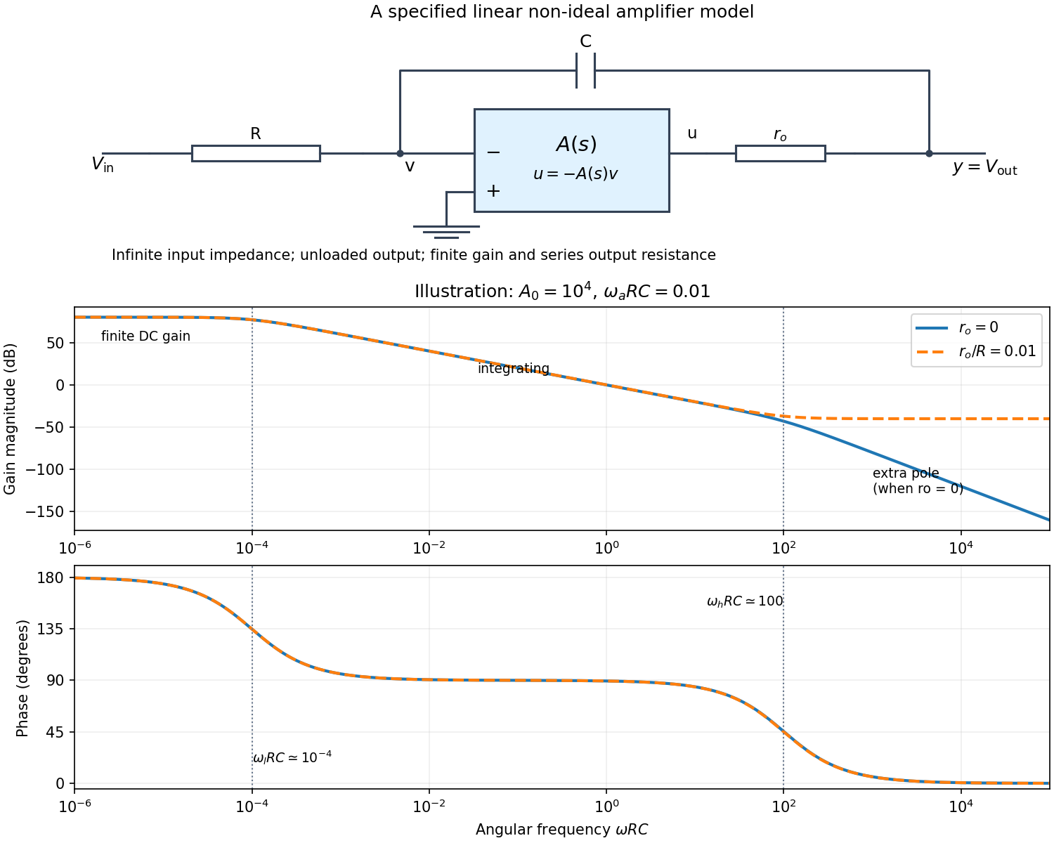
Writing Kirchhoff's current law at the input and output nodes givesThe second equation gives $y=(sC{r}_o-A)v/(1+sC{r}_o)$. Substitution in the first gives the general transfer functionFor sinusoidal phasors, set $s=i\omega$. The numerator and denominator are complex, so the magnitude gives the amplitude ratio and their arguments give the relative phase.

The simplest model takes $r_o=0$ and a constant finite gain $A_0>0$. It givesThus below ${\omega }_l=[(1+A_0)RC{]}^{-1}$ the amplifier has gain magnitude $A_0$ and inversion. Above that frequency it approaches an integrator with magnitude $A_0/[(1+A_0)\omega RC]\simeq 1/(\omega RC)$ and phase $+90^{\circ }$. Constant finite gain by itself predicts no further high-frequency turnover.

For a more realistic sketch, use the standard dominant-pole open-loop gain $A(s)=A_0/(1+s/{\omega }_a)$, still with $r_o=0$. ThenThe exact frequency response isAssuming $A_0\gg 1$ and $A_0{\omega }_{a}RC\gg 1$, the turnover frequencies are well separated: ${\omega }_l\simeq 1/(A_{0}RC)$ and ${\omega }_h\simeq A_0{\omega }_a$, the approximate unity-gain angular frequency of the amplifier. The regimes arewith magnitude slopes $0,-20,-40\mathrm{dB}$ per decade and smooth phase transitions. This is the solid curve in the figure; $180^{\circ }$ and $-180^{\circ }$ denote the same phase.

If finite $r_o$ is retained and $A(i\omega )\to 0$, the general expression instead approaches $r_o/(R+r_o)$ at very high frequency: the capacitor couples the input to the output through a passive voltage divider. The dashed curve illustrates that eventual feedthrough. Other amplifier poles or an external load would alter the response again. No particular values of $A_0,{\omega }_a,r_o$ are given in the paper, so the numerical sketch is illustrative and the general expression states the model dependence explicitly.

A chi-squared test compares squared deviations with the size expected from the assumed random errors. For independent observations with a normal distribution $y_i$ with known standard deviations ${\sigma }_i$ and predictions ${\mu }_i(\theta )$, useFor a correct fixed model, the standardized independent residuals are unit-variance normal distributions, so $Q$ has a chi-squared distribution with $\nu =N$. Fitting $p$ independent linear parameters removes $p$ residual directions, giving $\nu =N-p$. This distribution is exact for a full-rank linear model with known errors with a normal distribution; it is an approximation for many nonlinear fits. With known correlated errors with a multivariate normal distribution, replace the sum by $Q={\mathbf{r}}^{\mathsf{T}}{\Sigma }^{-1}\mathbf{r}$, where $\Sigma$ is the covariance matrix and its rank and fitted constraints determine the available statistical degrees of freedom.

Under the null hypothesis, $\mathbb{E}Q=\nu$ and $\mathrm{Var}Q=2\nu$. The reduced statistic $Q/\nu$ should therefore be near one, with standard deviation $\sqrt{2/\nu }$, rather than equal to one exactly. An upper-tail p-value isCompare it with a significance threshold chosen in advance. A small value indicates tension with the model together with its error assumptions; it can arise from a wrong mean model, underestimated uncertainties or neglected correlations. An unusually small statistic can suggest overestimated uncertainties, correlations or overfitting. A p-value is not the probability that the model is true, and failure to reject is not proof of the model.

For counts in categories, the Pearson form is $Q={\sum }_{j=1}^k(O_j-E_j{)}^2/E_j$. Its chi-squared distribution is an asymptotic approximation requiring adequate expected counts. For a fixed-total multinomial sample there is one normalization constraint, so the usual statistical degrees of freedom are $k-1-p$ after fitting $p$ other parameters. Independent Poisson bins instead start with $k$ statistical degrees of freedom before parameters are fitted. Sparse counts require an appropriate count likelihood or a calibrated exact or simulation-based test; plugging tiny expected counts into the asymptotic formula is unreliable. The error model, binning, fitted parameters and chosen test must therefore be reported with the result.

Temperature changes affect measurements through several routes. Thermal expansion changes lengths and alignments; temperature-dependent resistance and refractive index change electrical and optical calibrations; temperature differences between dissimilar junctions generate Seebeck effect voltages. These slow environmental changes are distinct from unavoidable equilibrium thermal fluctuations and Johnson-Nyquist noise. A useful strategy identifies the coupling to the measured signal before choosing a remedy.

Reduce environmental coupling by enclosing the apparatus against drafts, using thermal insulation and radiation shields, isolating heat sources, and minimizing dissipated power. A vacuum enclosure suppresses convection but leaves thermal conduction and thermal radiation paths to control. A large heat capacity reduces rapid temperature excursions. In a simple thermal model with heat capacity $C_T$ and thermal conductance $G_T$ to a reservoir, the relaxation time is $C_T/G_T$, so adequate settling time is necessary after changing the apparatus. A temperature sensor close to the sensitive element and stable negative feedback heating or cooling can regulate its temperature; poorly placed sensors or excessive feedback gain can leave gradients or cause oscillations.

Electrical thermal noise has the classical low-frequency one-sided voltage power spectral densityfor a resistor measured over a flat bandwidth $B$ without significant loading. More generally replace $B$ by the effective noise bandwidth. Lower temperature or narrower bandwidth reduces the noise, and resistance choices must account for source loading and the amplifier's own voltage and current noise. A lock-in amplifier uses modulation and narrowband detection to reject much low-frequency drift and out-of-band noise, while thermal noise inside the accepted band remains. Temperature stabilization does not remove equilibrium fluctuations.

Use a matched reference or differential bridge to reject common environmental changes. Keep junctions isothermal and choose matched materials to reduce thermoelectric offsets. For a resistance measurement, reversing a small test current separates a stable offset from the wanted voltage:Reversal must be fast enough that the offset stays approximately fixed, with enough settling time and sufficiently little self-heating. Recording the sample temperature permits a measured calibration slope $dS/dT$ to correct a signal to a reference temperature; the correction's calibration and thermometer uncertainties must be propagated. Independent white noise fluctuations decrease under averaging, whereas correlated temperature drift may not decrease as the inverse square root of the number of readings. Temperature records and repeated reference measurements help distinguish the two.

Digital acquisition converts a continuous voltage signal into timed numerical samples. A practical chain is a suitably buffered and amplified sensor signal, an analogue anti-aliasing filter, a sampling or sample-and-hold stage, an analog-to-digital converter, and a clocked data-storage system. Choose the gain so that the interesting variation uses the available input range without clipping. Finite input impedance can load a sensor, so an appropriate buffer or operational amplifier may be needed.

Sampling makes time discrete. If the conditioned signal is confined below frequency $f_{\max }$, choose a sampling rate $f_s>2f_{\max }$, allowing a transition band for the physical filter. The Nyquist–Shannon sampling theorem permits ideal reconstruction of a suitably bandlimited function from exact samples. Without filtering, components separated by integer multiples of $f_s$ have identical samples; in particular real sinusoids at $f$ and $f_s-f$ can be indistinguishable. This aliasing cannot generally be undone by later digital filtering. Oversampling can ease filter design, but does not replace the requirement to suppress unwanted high-frequency content before sampling.

Amplitude quantization is separate from sampling. A uniform $b$-bit converter covering voltage span $V_{\mathrm{span}}$ has step $q\simeq V_{\mathrm{span}}/2^b$. Rounding an in-range input gives the uniform-quantization error bound $|ϵ|\le q/2$. If the rounding errors can additionally be modeled as uniform and uncorrelated, their standard deviation is $q/\sqrt{12}$. This statistical estimate is not a guarantee for a constant input or a coherent periodic signal. More bits increase resolution, but accuracy also depends on voltage-reference calibration, offset, gain error, nonlinearity and electronic noise. Out-of-range signals clip and invalidate the rounding bound.

Clock quality matters too. Timing jitter $\delta t$ gives a voltage error approximately $(dV/dt)\delta t$; for a sinusoid its scale grows with $2\pi f{V}_p{\sigma }_t$. A clock calibration error biases measured frequencies and time intervals. Simultaneous multichannel signals need known relative timing, and the sampling and analogue settling times must be appropriate to the signal bandwidth.

For $n_c$ channels the raw recording rate is approximately $n_c{f}_{s}b$ bits per second, before overhead, so storage and sustained transfer speed must prevent missing data. Store units, channel identities, timestamps, sampling rate, input ranges and calibration information along with the readings. Preserve the original samples when applying digital filters or other processing. Averaging can improve precision for independent fluctuating errors, but cannot restore aliased frequencies, clipped peaks or a fixed rounding bias. Digital recording makes reproducible analysis and transmission possible when its sampling, amplitude and timing limitations are all controlled.