Write and use the Heisenberg uncertainty relation separately in the three Cartesian directions. Since a position coordinate is confined to an interval of length , Popoviciu's inequality on variances gives . Consequently , and the expectation value of the kinetic energy obeysThus an uncertainty-based lower estimate is . This confinement energy bound from position support is not sharp: the exact ground-state energy for a cubical infinite square well is . The Heisenberg uncertainty principle establishes the confinement scale ; identifying a box size with an approximate position standard deviation changes its numerical coefficient.
The rotational kinetic energy is . For a three-dimensional linear rigid rotor, angular momentum operator replaces the squared magnitude by , where . HenceThe three lowest distinct energy levels are thereforeTheir magnetic quantum degeneracy values are . A single moment of inertia specifies this rigid rotor model; an arbitrary asymmetric body would require its other principal moments.
Inside the barrier, the stationary Schrödinger equation gives an exponentially decaying wavefunction with inverse penetration lengthThe amplitude falls approximately as , so the leading exponential estimate for the transmission probability isFor comparison, wavefunction matching at a finite potential step at both edges gives the rectangular-barrier tunnelling probabilityThe difference is the interface prefactor: for an opaque barrier it is . Both give a transmission of order ; the first is the requested exponential estimate.
Ohm's law gives the mean electric currentFor an estimate, assume the shot noise counting model: electron transfers are independent, so the number recorded in an interval has a Poisson distribution with expectation value and variance . One measurement has relative standard deviation . Averaging independent intervals reduces this to , soabout minutes in total.
This is a one-standard deviation, shot noise estimate. A resistance and mean voltage alone do not specify the actual current fluctuations: a real resistor also has Johnson-Nyquist noise, and electron-transfer correlations can change the shot noise. Its temperature, measurement bandwidth and noise model would be needed for an unconditional acquisition time.
For independent small uncertainties interpreted as standard deviations, propagation of uncertainty givesThe angular uncertainty is in radians. Since , the allowed angular contribution to the fractional uncertainty of the numerical aperture is only . ThereforeThe uncertainty in the refractive index already contributes . If the quoted errors instead mean strict worst-case bounds, first-order absolute errors must be added rather than added in quadrature; that convention would require . The result uses the usual independent statistical-error convention.
Write , with the Pauli matrices. Direct multiplication gives , and henceFor the products in the other order,Their difference gives the angular momentum commutation relationsThe first identity corresponds to the spin one-half value with .
In the eigenbasis, let a candidate eigenvector be . The eigenvalue equation is and , so a nonzero vector requires . Choosing normalized phases givesThe two spin eigenstates are orthogonal, as required for distinct eigenvalues of a self-adjoint operator.
Put , including its sign. The initial vector is the eigenstate of ; it is not an energy eigenstate of . In terms of the spin eigenstates found above, . Each energy eigenstate acquires its own unitary time evolution phase:Equivalently, follows from . The Born rule givesThe expectation value of the spin angular momentum is , a rotation around the axis. Its direction follows the specified sign of the Hamiltonian; changing the magnetic coupling sign reverses the precession.
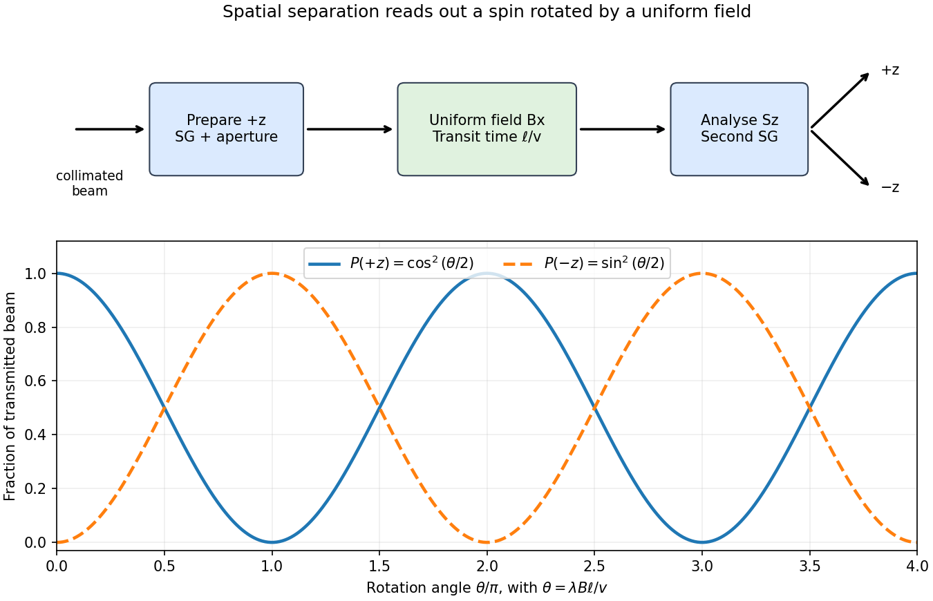
A Stern-Gerlach experiment uses an oven and slits to produce a collimated atomic beam, conventionally of neutral silver atoms, and sends it through an inhomogeneous magnetic field onto a position-sensitive detector. The unpaired outer electron supplies the effective spin one-half magnetic dipole moment; neutral atoms avoid the ordinary Lorentz deflection of a charged beam. For an analysing direction , the spatial gradient produces a force approximately . The resulting separated beam positions measure the allowed projections of angular momentum. A spin one-half beam gives two branches, rather than the continuous distribution expected from classical dipoles with arbitrary orientations. A uniform magnetic field can rotate a spin but does not itself provide this spatial separation.
To measure the rotation, first use a -directed Stern-Gerlach experiment and an aperture to transmit only the branch. Pass this prepared spin eigenstate through a region of approximately uniform field in the direction, then use a second analyser to separate and count the two populations. For a field region of length and beam speed , the precession angle is , and the predicted fractions areVarying or the transit time gives complementary oscillations, demonstrating coherent Larmor precession. Velocity selection and a sufficiently uniform rotation field keep different particles from accumulating different phases and washing out the contrast. Detection should compare the branch fractions after allowing for losses and analyser efficiency.
Use the nonrelativistic Coulomb potential energy , with the nucleus treated as fixed. Since the wavefunction has zero orbital angular momentum, its Laplacian isSubstituting into the time-independent Schrödinger equation givesFor a constant energy eigenvalue, the coefficient of must vanish. Therefore , where is the Bohr radius. Wavefunction normalization then requiresChoosing the irrelevant overall phase so that is real and positive gives . The remaining constant term is the hydrogen ground-state energyReplacing by the electron-nucleus reduced mass gives the usual finite-nuclear-mass refinement.
The normalized radial probability density givesConsequently the expectation value of the potential energy isHere the last equality uses . Since this is an energy eigenstate, , and so . The kinetic energy is positive because , in agreement with the virial theorem for a Coulomb potential.
The probability of finding the electron in a spherical shell is , soThis radial probability density, rather than the density per unit volume, determines the most probable radius. Its expectation value isFor its interior maximum, differentiate . The stationary condition givesThe density per unit volume is instead largest at the nucleus; including the spherical-shell volume factor is essential to the requested radial mode.
The nuclear beta decay is fast compared with the electronic orbital timescale. In the sudden approximation, the electronic wavefunction does not have time to change during the increase from to . The subsequent probability of a particular daughter energy eigenstate is therefore its squared overlap with the initial state.
For the final state, write and . The sudden hydrogenic charge change gives the amplitudeThusThe final states have spherical harmonics , whereas the initial state is proportional to . Their angular overlap vanishes by orthogonality. Accordingly in the ideal spherically symmetric sudden-change model. Nuclear recoil or interactions with the emitted particles can produce small corrections. This is an overlap selection rule for a sudden change, not a photon-induced electric dipole transition.
The infinite walls impose , and the interior time-independent Schrödinger equation is with . Its general solution is . The first boundary condition gives , and the second gives . A nonzero normalizable state needs ; would give the zero function.
Wavefunction normalization, , gives the infinite square well states and their energy eigenvalues:The wavefunctions vanish outside the well, and their full time dependence is .
The first two probability densities areBoth vanish at the walls. The ground state has one maximum at and no interior node. The first excited state has a node at and equal maxima at and .
For a finite square well whose exterior potential is , the exterior wavefunction decays as , where and is distance from the relevant edge. Wavefunction matching at a finite potential step makes the wavefunction and, for constant mass, its first derivative continuous. Thus the probability density is nonzero at the edges and has evanescent tails outside, the interior wavelength increases, and the energy levels are lower than for infinite walls at the same positions. Reflection symmetry still gives an even ground state and odd first excited state about the center, when both are bound. A shallow well may not support that excited bound state at all.
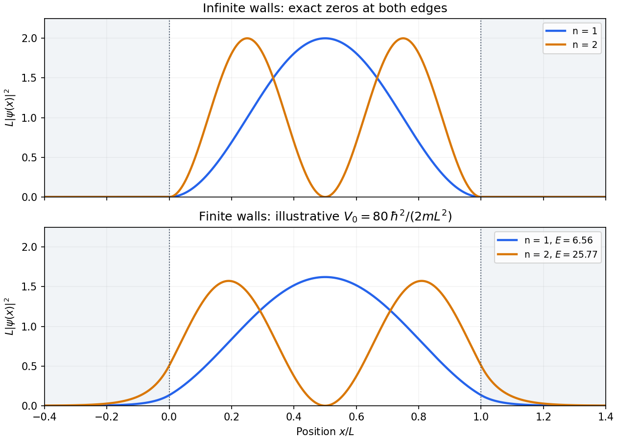
Lowest box-state densities and their evanescent tails for one finite-depth example
. Details. Choose the two real energy eigenstates in part (a) and take their coefficients to be in phase initially. A different initial relative phase only shifts the oscillation in time. The normalized quantum superposition isOrthogonality removes the cross terms in the energy expectation value, soFor position, the diagonal matrix elements equal by reflection symmetry, but the off-diagonal element is nonzero. Using the product-to-sum identity and givesTherefore the equal superposition of the first two box states hasThe amplitude is , and the ordinary frequency is . The motion of the mean position is an interference effect between distinct energies, while their populations, and hence the mean energy, remain fixed.
The boundary force in an infinite square well is obtained from the kinetic momentum flux at each wall. With , the derivatives of the state in part (c) areThe outward force magnitudes are . Taking positive force to mean rightwards, the forces exerted by the particle on the walls areBoth point outwards at all times, but their magnitudes oscillate out of phase. This force formula follows directly by differentiating the mean particle momentum and integrating the interior Schrödinger equation by parts: . As a check, the net force on the particle is , the opposite of the net force on the two walls.
A classical particle of energy transfers momentum in each collision with a particular wall, and returns to that wall after . Its mean outward force on that wall isThus the time averages agree separately at each wall, although the classical force consists of collision impulses and the quantum expectation varies continuously. Constant mean energy alone does not make the instantaneous quantum wall forces constant; their unequal instantaneous values supply the oscillation of .
Let and , so and . The canonical commutation relation givesHence . Similarly,Using the product rule for a commutator, , givesThus is the number operator, while and are the annihilation operator and creation operator.
The commutators implyThus any nonzero resulting vector is the adjacent energy eigenstate. Since and , their squared norms areChoosing consistent phases for the eigenstates yieldsThe vanishing last expression terminates the lowering sequence at the ground state, rather than introducing a negative-energy oscillator state.
In the position representation , so becomesIntegrating and using the Gaussian integral for wavefunction normalization givesThe creation operator gives , and thereforeIts norm is one since . Moreover is even and is odd, so the overlap integrand is odd and integrable. Integration over the whole real line gives , establishing orthogonality.
Inverting the definitions of the creation operator and annihilation operator gives . Their actions and the orthogonality of the oscillator energy eigenstates giveThus the electric dipole transition selection rule iswith the lower alternative absent for . The field exchanges one oscillator quantum in first-order dipole coupling. For a long weak monochromatic drive, its frequency must also be resonant with the level separation, here , to give a substantial transition probability. Higher-order multiphoton processes are beyond the stated single-position-matrix element approximation.
A localized quantum particle is described by a wave packet: a coherent quantum superposition of momentum components, rather than a single delocalized plane wave. The Born rule assigns the position probability density . A useful normalized initial Gaussian wave packet isIts mean position and momentum are and , and its standard deviations satisfy , . This unchirped initial state saturates the Heisenberg uncertainty relation.
For a free particle, the momentum-space Schrödinger equation multiplies each amplitude by . The inverse Fourier transform is a Gaussian integral, giving the free Gaussian wave packet evolutionOne way to obtain this expression explicitly is to write the initial momentum amplitude as proportional to , multiply by the free evolution phase and complete the square in . Taking the modulus squared removes the position-dependent phase and leavesThe expectation value follows uniform classical motion while the density spreads. A narrower initial packet needs a wider momentum distribution and therefore spreads more rapidly. At long times its width grows linearly with ; its variance grows quadratically, unlike the linear variance growth of ordinary diffusion. The probability continuity equation preserves total probability despite the decreasing peak height. The mean momentum and the mean energy remain constant, since the momentum populations do not change.
The same result has a wave interpretation. For a free nonrelativistic particle , so the group velocity is , equal to at the packet center. The curvature makes different momentum components travel with different group velocities, producing dispersion. The phase velocity is for this energy convention and does not describe the motion of the envelope. The evolving quadratic spatial phase is essential to the spreading; a density snapshot alone does not specify the full quantum state.
A freely spreading Gaussian wave packet remains a pure Gaussian state but develops position-momentum correlations. Its symmetrized covariance is . ConsequentlyEquality in the Robertson-Schrödinger uncertainty relation survives at every time, whereas the simpler product equals only initially. A chirped Gaussian wave packet can already have . More generally, gives . A sufficiently negative initial covariance permits initial contraction before subsequent spreading.
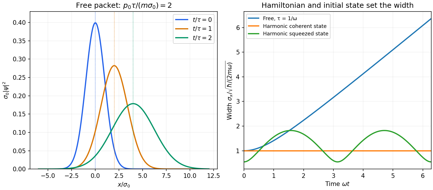
A potential energy changes this behavior. A quadratic potential preserves the Gaussian form because the evolution of position and momentum is linear. For a quantum harmonic oscillator, the Gaussian covariance in a harmonic potential isA coherent state has , and zero centered covariance. Its width is constant, and its center follows . In oscillator notation its coherent state label rotates as , apart from the common ground-energy phase of the state vector. A squeezed coherent state generally has a width that breathes at . Thus being Gaussian does not imply either free spreading or constant width; the Hamiltonian operator and initial covariance determine the result.
For a general nonquadratic potential, different parts of the packet experience different nonlinear forces, and an initially Gaussian profile need not remain Gaussian. Ehrenfest theorem gives the exact relations and . Replacing the last mean by is exact for a quadratic potential and approximate for a packet narrow compared with the scale on which the force varies. This connects packet motion to the correspondence principle without treating a quantum state as a definite classical path. Scattering can split a packet into reflected and transmitted components, while confinement can produce oscillations and interference between discrete energy eigenstates. Their relative phases evolve even when their populations remain constant. Localization, spreading and coherent motion all follow from the same linear unitary time evolution.
The orbital angular momentum of a particle is the operator , with in the position representation. Its angular momentum commutation relations areThus one may specify and one component, conventionally , simultaneously. One generally cannot assign sharp values to all three components, because they do not commute. The common angular eigenfunctions are the spherical harmonics:For a scalar orbital wavefunction, single-valuedness in the azimuthal angle gives integer , and regularity on the sphere and termination of the ladder give integer . Half-integer angular momenta describe intrinsic spin rather than scalar orbital motion.
The ladder operators obey . Their normalized action isThe coefficient vanishes at the top or bottom of the multiplet. Its squared magnitude follows from , and positivity of the resulting norm constrains the allowed values.
For a central potential, the Hamiltonian commutes with and every component of . Stationary states can be separated as , and rotational symmetry makes the energy independent of , giving a quantum degeneracy at fixed radial label and . Additional degeneracy between distinct values requires additional structure, as in the Coulomb potential. The parity of is . These results organize atomic orbitals and their selection rules. They describe quantized rotation and symmetry, without assigning the electron a classical orbit or a simultaneously definite three-component angular momentum vector.
In the Schrödinger picture, a time-independent Hamiltonian gives , where . The Heisenberg picture transfers this evolution to each observable:Both pictures give the same probabilities and expectation values. Differentiating yields the Heisenberg equation of motionThe last term is an explicit change of the measured operator. If it is absent and , the observable is conserved.
The corresponding classical equation is . The correspondence principle relates the Poisson bracket to , with suitable operator ordering and a classical limit. For , the canonical commutation relation givesTaking means gives Ehrenfest theorem. Its second equation contains , which need not equal . A narrow wave packet in a slowly varying force field can follow the classical equations approximately; a quadratic potential makes the equality exact for the means.
For a quantum harmonic oscillator, direct solution gives and . These have the classical form as operator identities. A coherent state supplies a localized center moving on the classical orbit, whereas an energy eigenstate has stationary density and , even at large excitation. Thus large quantum numbers alone do not create a localized classical trajectory. Classical behavior also concerns state preparation, relative fluctuations and the resolution of the measurements.
An observable is represented by a self-adjoint operator. For an ideal projective measurement, let be its spectral projector for outcome . The Born rule gives , or for a density matrix . Conditional on obtaining , the Lüders rule givesFor a degenerate outcome this projects onto the whole associated eigenspace, rather than arbitrarily selecting a vector within it. An immediate repeated ideal measurement returns the same outcome, provided there is no intervening evolution or disturbance.
Commuting finite-dimensional observables admit a common orthonormal eigenbasis; their projectors commute and ideal joint measurements are compatible. Noncommuting observables generally have no complete common eigenbasis, and measurement order can affect the subsequent statistics. Particular common eigenvectors can nevertheless exist, so a nonzero commutator does not mean that every state has a nonzero uncertainty in both quantities.
For a quantitative constraint, apply the Cauchy-Schwarz inequality to and . The imaginary part of their inner product is , giving the Robertson uncertainty principleThe canonical commutation relation gives . Retaining the real part of the same inner product gives the stronger Robertson-Schrödinger uncertainty relation, including a covariance term. These are constraints on the preparation of a quantum state, not simply statements about a poorly calibrated instrument.
A sequential spin one-half example makes the change in statistics explicit. Prepare . An immediate measurement is certainly positive. If an measurement is inserted first, its outcomes each have probability and leave states . Each then yields either result with probability , so the final positive fraction is . The change reflects projection onto incompatible spin eigenstates, even with ideal measuring apparatus. The theory of measurement in quantum mechanics allows more general state-update rules, but the operator description and the Born rule still constrain their probabilities.
An ideal operational amplifier has infinite differential open-loop gain, infinite input impedance, zero output impedance, unlimited bandwidth and slew rate, and zero input offset voltage, input bias current and intrinsic noise. The idealized model has no finite output-swing or output-current limit.
The usual circuit rules areThe first follows from infinite input impedance. The second follows because a finite output requires as the open-loop gain tends to infinity. It is a virtual equality of potentials, not a conducting connection between the inputs. It cannot be imposed for open-loop operation or after an amplifier reaches its supply rails.
Let be the inverting-input potential. The non-inverting input is grounded, so the ideal operational amplifier rules give and no input current. Kirchhoff's current law at that node therefore givesIntegrating from an initial time ,This op amp integrator performs inverted time integration; the initial voltage across the capacitor supplies the integration constant. For zero initial conditions its transfer function is . In sinusoidal steady state, with the convention ,For example, a cosine input produces a negative sine output after its constant component is set. The additional inversion makes the phase modulo , rather than the of non-inverting integration.
Any direct-current component of the input produces an output ramp. The input offset voltage and input bias currents of a real operational amplifier therefore charge the feedback capacitor until the output saturates. Even the desired signal can exceed the available output swing when integrated for too long. Initial capacitor charge also introduces an unknown integration constant.
Place a large resistor in parallel with the feedback capacitor. The idealized transfer function then becomesIts finite direct-current gain supplies a return path and bounds the response to a small offset; it approximates when . The chosen gain must still keep offsets within the output range. A reset switch across the capacitor can set the initial charge, while low-offset amplifiers, bias compensation and input offset adjustment reduce drift. Useful integration also requires frequencies below the amplifier's own response limit.
A real operational amplifier has large but finite, frequency-dependent open-loop gain; the gain falls and its phase changes at higher frequencies. Finite bandwidth and slew rate constrain small-signal and large-signal responses respectively. There are also finite input impedance and output impedance, nonzero input bias currents and input offset voltage, and internally generated noise. Offset and bias can drift with temperature.
The output is limited by the supply voltages and output-current capability, and the inputs have a permitted common-mode range. Rejection of common-mode and supply changes is finite. Consequently need not vanish exactly, and neither the virtual-ground approximation nor linear gain formulas apply after saturation. For the calculation below the stipulated infinite input impedance removes the input loading currents, while finite gain and optionally finite output resistance are retained.
A non-ideal amplifier is not specified by infinite input impedance alone: its open-loop gain and output impedance must also be modeled. Take its internal controlled output to be , where is the inverting-input potential, and place a resistance between and the actual output . The non-inverting input remains grounded; assume no external load. This gives an explicit finite-gain operational-amplifier integrator model.
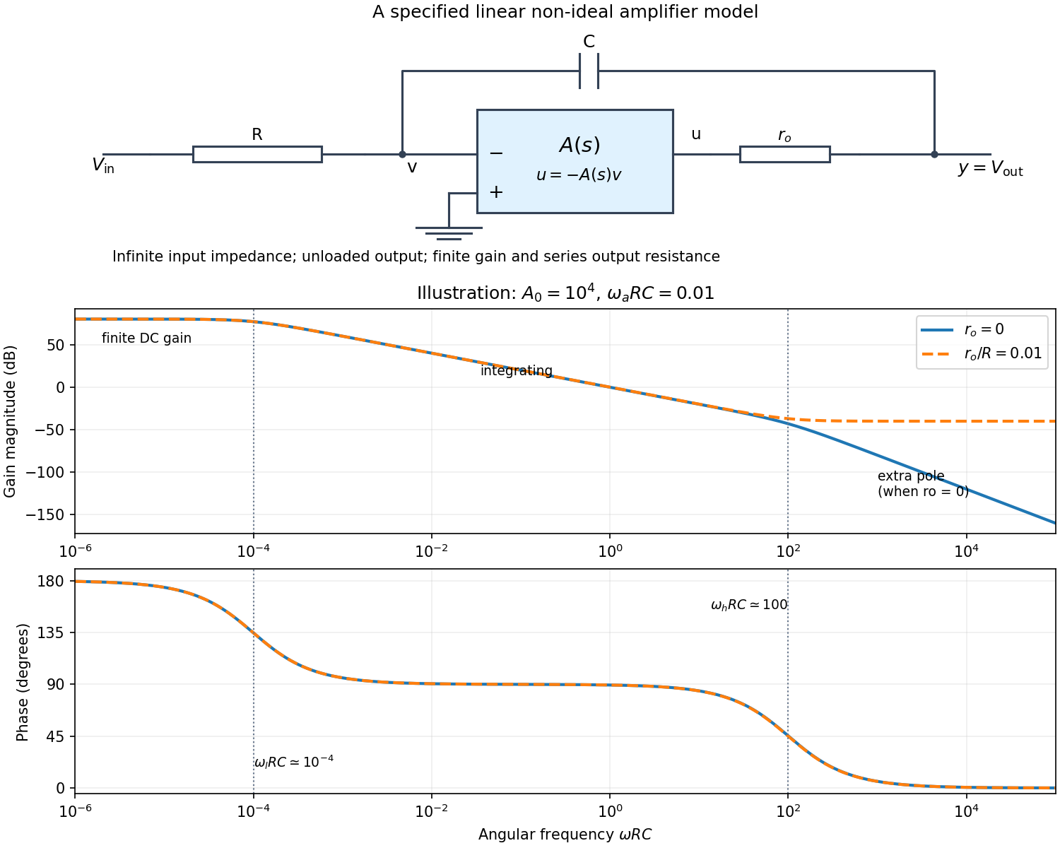
Writing Kirchhoff's current law at the input and output nodes givesThe second equation gives . Substitution in the first gives the general transfer functionFor sinusoidal phasors, set . The numerator and denominator are complex, so the magnitude gives the amplitude ratio and their arguments give the relative phase.
The simplest model takes and a constant finite gain . It givesThus below the amplifier has gain magnitude and inversion. Above that frequency it approaches an integrator with magnitude and phase . Constant finite gain by itself predicts no further high-frequency turnover.
For a more realistic sketch, use the standard dominant-pole open-loop gain , still with . ThenThe exact frequency response isAssuming and , the turnover frequencies are well separated: and , the approximate unity-gain angular frequency of the amplifier. The regimes arewith magnitude slopes per decade and smooth phase transitions. This is the solid curve in the figure; and denote the same phase.
If finite is retained and , the general expression instead approaches at very high frequency: the capacitor couples the input to the output through a passive voltage divider. The dashed curve illustrates that eventual feedthrough. Other amplifier poles or an external load would alter the response again. No particular values of are given in the paper, so the numerical sketch is illustrative and the general expression states the model dependence explicitly.
A chi-squared test compares squared deviations with the size expected from the assumed random errors. For independent observations with a normal distribution with known standard deviations and predictions , useFor a correct fixed model, the standardized independent residuals are unit-variance normal distributions, so has a chi-squared distribution with . Fitting independent linear parameters removes residual directions, giving . This distribution is exact for a full-rank linear model with known errors with a normal distribution; it is an approximation for many nonlinear fits. With known correlated errors with a multivariate normal distribution, replace the sum by , where is the covariance matrix and its rank and fitted constraints determine the available statistical degrees of freedom.
Under the null hypothesis, and . The reduced statistic should therefore be near one, with standard deviation , rather than equal to one exactly. An upper-tail p-value isCompare it with a significance threshold chosen in advance. A small value indicates tension with the model together with its error assumptions; it can arise from a wrong mean model, underestimated uncertainties or neglected correlations. An unusually small statistic can suggest overestimated uncertainties, correlations or overfitting. A p-value is not the probability that the model is true, and failure to reject is not proof of the model.
For counts in categories, the Pearson form is . Its chi-squared distribution is an asymptotic approximation requiring adequate expected counts. For a fixed-total multinomial sample there is one normalization constraint, so the usual statistical degrees of freedom are after fitting other parameters. Independent Poisson bins instead start with statistical degrees of freedom before parameters are fitted. Sparse counts require an appropriate count likelihood or a calibrated exact or simulation-based test; plugging tiny expected counts into the asymptotic formula is unreliable. The error model, binning, fitted parameters and chosen test must therefore be reported with the result.
Temperature changes affect measurements through several routes. Thermal expansion changes lengths and alignments; temperature-dependent resistance and refractive index change electrical and optical calibrations; temperature differences between dissimilar junctions generate Seebeck effect voltages. These slow environmental changes are distinct from unavoidable equilibrium thermal fluctuations and Johnson-Nyquist noise. A useful strategy identifies the coupling to the measured signal before choosing a remedy.
Reduce environmental coupling by enclosing the apparatus against drafts, using thermal insulation and radiation shields, isolating heat sources, and minimizing dissipated power. A vacuum enclosure suppresses convection but leaves thermal conduction and thermal radiation paths to control. A large heat capacity reduces rapid temperature excursions. In a simple thermal model with heat capacity and thermal conductance to a reservoir, the relaxation time is , so adequate settling time is necessary after changing the apparatus. A temperature sensor close to the sensitive element and stable negative feedback heating or cooling can regulate its temperature; poorly placed sensors or excessive feedback gain can leave gradients or cause oscillations.
Electrical thermal noise has the classical low-frequency one-sided voltage power spectral densityfor a resistor measured over a flat bandwidth without significant loading. More generally replace by the effective noise bandwidth. Lower temperature or narrower bandwidth reduces the noise, and resistance choices must account for source loading and the amplifier's own voltage and current noise. A lock-in amplifier uses modulation and narrowband detection to reject much low-frequency drift and out-of-band noise, while thermal noise inside the accepted band remains. Temperature stabilization does not remove equilibrium fluctuations.
Use a matched reference or differential bridge to reject common environmental changes. Keep junctions isothermal and choose matched materials to reduce thermoelectric offsets. For a resistance measurement, reversing a small test current separates a stable offset from the wanted voltage:Reversal must be fast enough that the offset stays approximately fixed, with enough settling time and sufficiently little self-heating. Recording the sample temperature permits a measured calibration slope to correct a signal to a reference temperature; the correction's calibration and thermometer uncertainties must be propagated. Independent white noise fluctuations decrease under averaging, whereas correlated temperature drift may not decrease as the inverse square root of the number of readings. Temperature records and repeated reference measurements help distinguish the two.
Digital acquisition converts a continuous voltage signal into timed numerical samples. A practical chain is a suitably buffered and amplified sensor signal, an analogue anti-aliasing filter, a sampling or sample-and-hold stage, an analog-to-digital converter, and a clocked data-storage system. Choose the gain so that the interesting variation uses the available input range without clipping. Finite input impedance can load a sensor, so an appropriate buffer or operational amplifier may be needed.
Sampling makes time discrete. If the conditioned signal is confined below frequency , choose a sampling rate , allowing a transition band for the physical filter. The Nyquist–Shannon sampling theorem permits ideal reconstruction of a suitably bandlimited function from exact samples. Without filtering, components separated by integer multiples of have identical samples; in particular real sinusoids at and can be indistinguishable. This aliasing cannot generally be undone by later digital filtering. Oversampling can ease filter design, but does not replace the requirement to suppress unwanted high-frequency content before sampling.
Amplitude quantization is separate from sampling. A uniform -bit converter covering voltage span has step . Rounding an in-range input gives the uniform-quantization error bound . If the rounding errors can additionally be modeled as uniform and uncorrelated, their standard deviation is . This statistical estimate is not a guarantee for a constant input or a coherent periodic signal. More bits increase resolution, but accuracy also depends on voltage-reference calibration, offset, gain error, nonlinearity and electronic noise. Out-of-range signals clip and invalidate the rounding bound.
Clock quality matters too. Timing jitter gives a voltage error approximately ; for a sinusoid its scale grows with . A clock calibration error biases measured frequencies and time intervals. Simultaneous multichannel signals need known relative timing, and the sampling and analogue settling times must be appropriate to the signal bandwidth.
For channels the raw recording rate is approximately bits per second, before overhead, so storage and sustained transfer speed must prevent missing data. Store units, channel identities, timestamps, sampling rate, input ranges and calibration information along with the readings. Preserve the original samples when applying digital filters or other processing. Averaging can improve precision for independent fluctuating errors, but cannot restore aliased frequencies, clipped peaks or a fixed rounding bias. Digital recording makes reproducible analysis and transmission possible when its sampling, amplitude and timing limitations are all controlled.
Build a narrow-band wave packet from plane waves with wavenumbers close to :The Taylor expansion of the dispersion relation is , where . Put to obtainThe carrier's wave phase travels at the phase velocity , while the envelope has constant shape at constant . Its group velocity is thereforeThe approximation neglects higher derivatives of the dispersion relation. Those derivatives cause the wave packet to spread or distort over sufficiently long propagation times; the result describes the local envelope speed of a sufficiently narrow band.
Assume a massless junction and common tension . The characteristic impedance of a stretched string is , where is its linear mass density. The displacement reflection coefficient is , so the reflected fraction of power isSet . The positive solutions are , which are reciprocals. Thus the string density ratio for prescribed reflected power isThe impedance ratio is about , rather than the required density ratio. Reversing which string is on the incident side changes the reflected displacement sign but not the reflected power fraction.
A Michelson interferometer splits a collimated beam at a partially reflecting beam splitter. Two mutually perpendicular arms reflect from mirrors and recombine at the same beam splitter; the superposed returning beams produce interference fringes at the detector. Translate one mirror along its arm while holding the other fixed.
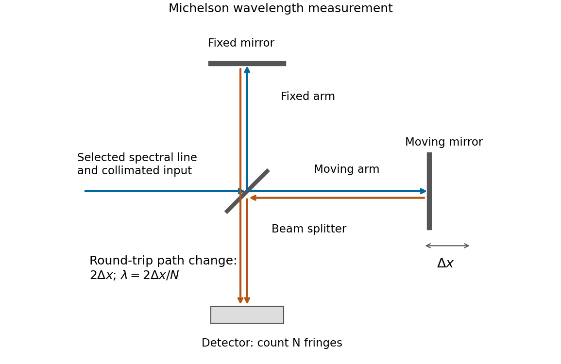
If that mirror moves a measured distance , the round-trip optical path difference changes by in air, approximated as vacuum. Every change of one wavelength moves one complete bright-dark-bright fringe cycle past a fixed detector point. Count such cycles to obtainUse a spectral line selected with a suitable optical filter, and count many interference fringes to reduce the fractional uncertainty of the distance and count. Keep the two arms within the source's optical coherence length and maintain overlap and alignment. If the vacuum wavelength is required for an arm filled with air of known refractive index , the corrected relation is at stable .
Take an abrupt equilibrium p-n junction with the p side at and the n side at . In the quasi-neutral bulk, electron holes are the majority carriers on the p side and Electrons are the majority carriers on the n side. With ionized dopant densities and nondegenerate statistics,where is the intrinsic carrier concentration. The semiconductor mass-action law applies at equilibrium. Both mobile populations are small in the depletion region compared with the dopant densities.
The charge and carrier density of an abrupt p-n junction must distinguish mobile populations from net charge. Diffusion leaves negatively charged ionized acceptor impurities on the p side and positively charged ionized donor impurities on the n side. Under the depletion approximation,The neutral bulks have large carrier densities but nearly zero net charge density. The electric field points from the positive donor region toward the negative acceptor region, balancing diffusion at equilibrium.
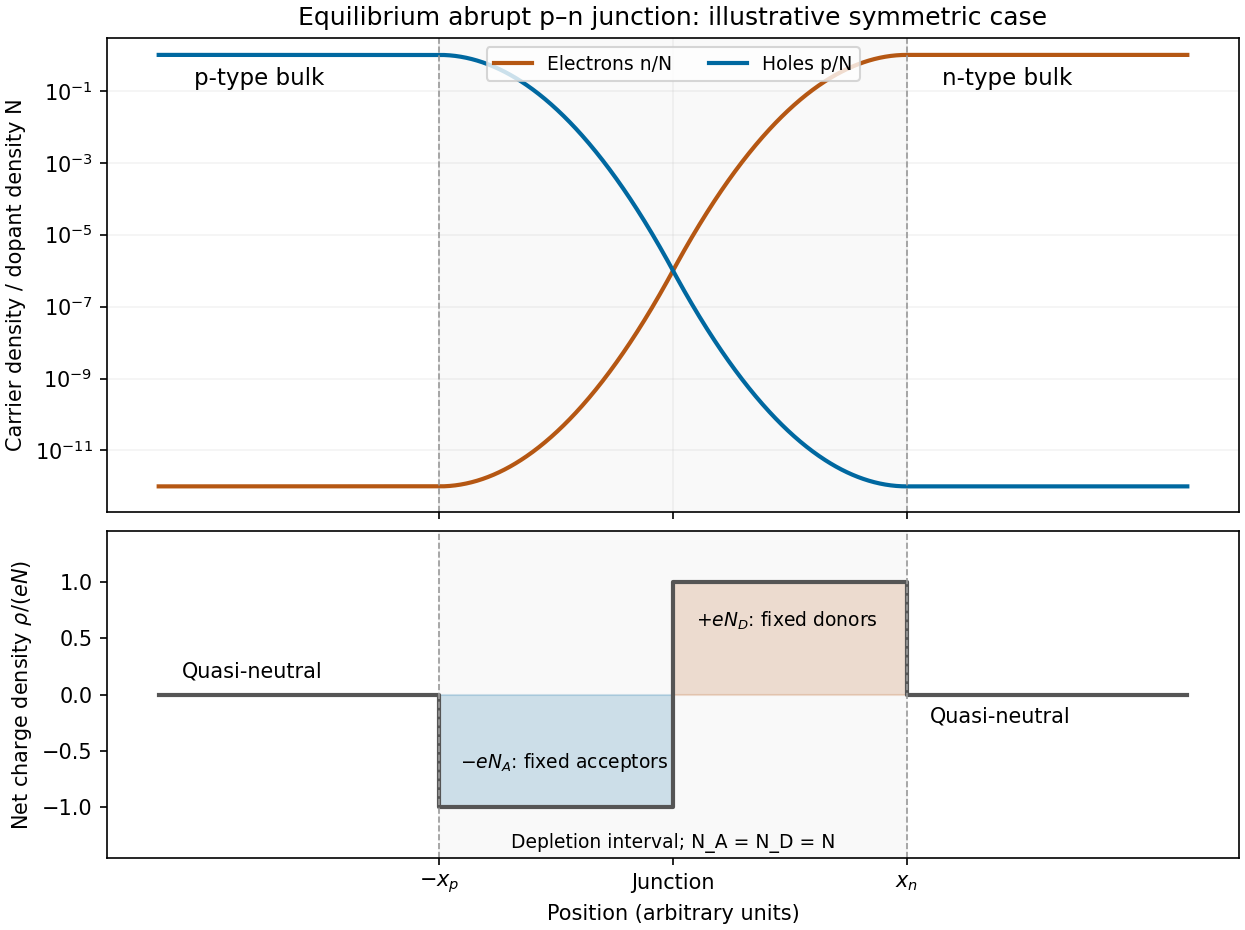
Illustrative equilibrium carrier densities and depletion-approximation net charge for a symmetric abrupt p-n junction
. Details. The figure uses equal dopant densities only to show a simple symmetric sketch. Generally the more lightly doped side has the wider depleted interval. The carrier profiles are smooth, whereas the step-shaped net charge density is the ideal depletion approximation.
Treat sodium as monovalent, with one mobile Electron per atom. Its mass density is , and its molar mass is . Using the Avogadro constant,The electron mobility relates the magnitude of drift velocity to electric field. The Drude model then givesUsing ,The inferred time is the momentum relaxation time. Identifying it with the mean time between collisions is the intended simple isotropic Drude model assumption; small-angle scattering need not relax directed momentum in a single event.
Draw the Fabry–Pérot etalon with parallel mirrors and an incident beam making internal angle with their normal. Every emerging transmitted contribution has undergone one more internal round trip than its predecessor.
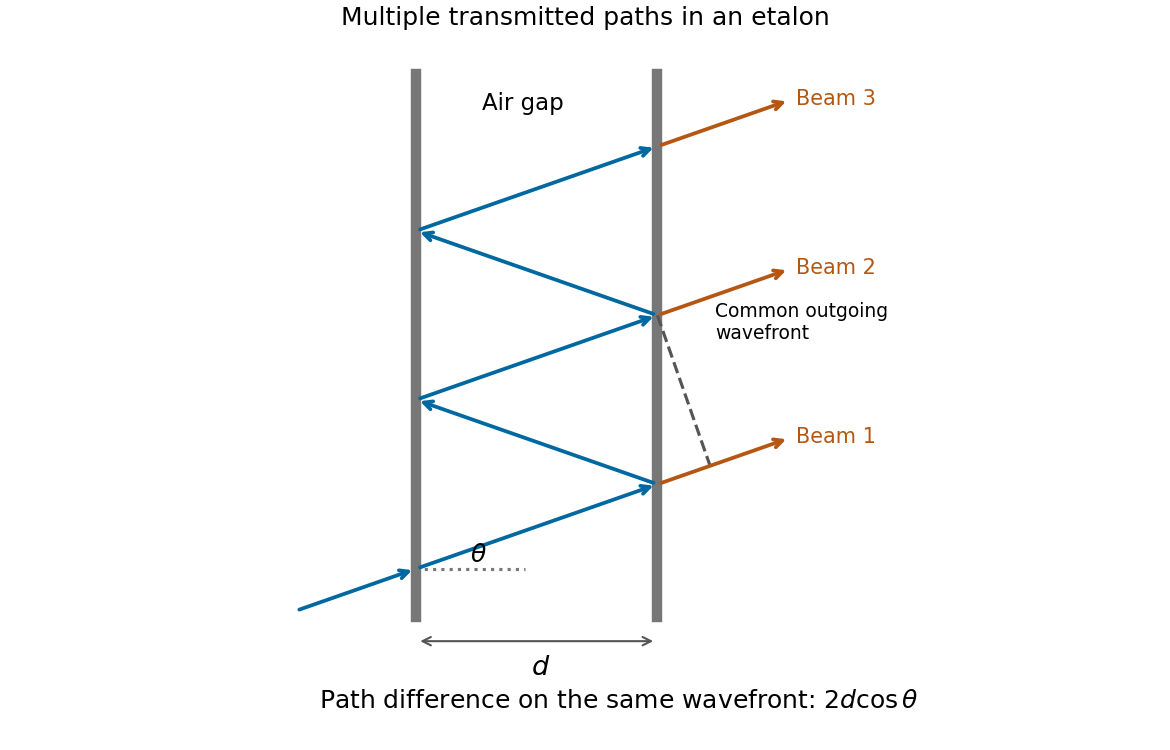


The extra internal path is , but successive contributions leave at laterally separated points, a distance apart. Comparing their phases on the same outgoing wavefront subtracts the path projection . Their net optical path difference in air isHence, in the reflection-phase convention implicit in the supplied transmission formula,For a gap of refractive index , replace by and use the vacuum wavelength. Coating reflection phases can add a round-trip offset; the expression above assumes that offset is absorbed in the resonance order, or is zero modulo as in the stated ideal model.
Write , keeping this coefficient distinct from the finesse . The transmission has maxima at . At a displacement from a maximum, its ratio to peak transmission is . Half maximum therefore requiresThis is the half-width in wave phase; the full width at half maximum is . Successive resonances are apart, so the exact ideal-model result isFor narrow peaks, , the small-angle approximation to the inverse sine givesThus the formula requested in the paper is the high-reflectivity approximation, not an exact identity at arbitrary . Ordinary half-maximum peaks exist only when , or ; below that threshold the transmission minimum never reaches half the peak. The prefactor cancels from this relative-width calculation.
Let , and . Requiring the separation to be at least times the measured full width at half maximum means a width no larger than , or a resolving power of approximately .
The etalon resolving power and order overlap constraints are particularly clear in frequency. Put . At normal incidence, the free spectral range is and the instrumental width is . ThusAvoiding ambiguity between the doublet and adjacent interference orders requires a free spectral range exceeding the doublet separation:Together these giveUsing the narrow-peak finesse from the previous part, gives , with a practical margin above that limiting value. At the exact limit, the gap between orders vanishes, so equality is not a sensible operating point.
One feasible ideal design is , , and . It has an approximate wavelength free spectral range of and instrumental width near the doublet. The doublet spacing is about widths. Even the spacing to the nearest replica of the other line exceeds widths in this example. If that latter separation is also required in general, impose the stronger condition , rather than just the two basic inequalities.
Such mirror reflectivities and submillimetre gaps are plausible for a high-quality Fabry–Pérot etalon. Flatness, parallelism, coating loss, angular spread, mechanical stability and source width limit the achieved finesse. A wavelength width of corresponds to a gap variation of order , so the ideal coating-limited estimate demands stringent uniformity. The paper expressly excludes intrinsic source broadening.
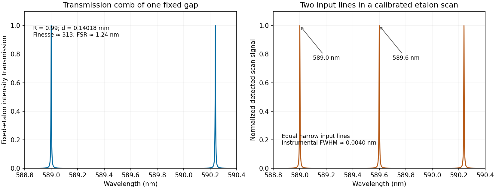
Calculated etalon transmission comb and a scanned doublet spectrum for an illustrative design meeting the width and order constraints
. Details. 
The first panel is the fixed etalon's transmission versus wavelength, a comb of resonances. It does not by itself have one peak at each sodium line. The second panel shows the two peaks obtained by scanning the etalon phase or gap and calibrating the scan to wavelength. A fixed-gap output spectrum is instead the incident spectrum multiplied by the transmission function. This distinction is needed to interpret a doublet measurement correctly.
A high-finesse Fabry–Pérot etalon obtains very narrow transmission peaks by summing many coherent round trips, allowing high resolving power with a compact optical path. It can transmit a substantial fraction of resonant light when coating absorption is small, and works well for precise relative line separations and narrow-line measurements. A diffraction grating may require many illuminated grooves to achieve the same resolving power.
The etalon's free spectral range is limited, and repeated orders cause ambiguity across a broad optical spectrum. It commonly needs scanning and an order-selecting optical filter or another dispersive element. Mirror alignment, flatness and illumination angle strongly affect peak positions and widths, and absorption lowers throughput. A diffraction grating instead separates a broad range of wavelengths spatially for simultaneous detection, although grating orders can also overlap. The preferred instrument depends on whether narrow-band precision or broad spectral coverage is the priority.
Articles were limited to the first 100 out of 164 total.
Articles by others on the same topic
There are currently no matching articles.