Take the natural logarithm of the exponential decay model. To keep the logarithm dimensionless, choose the reference rate and defineThen . With time measured in picoseconds, the slope has units and the intercept is dimensionless. A straight-line linear regression in these variables therefore estimates the inverse mean lifetime and logarithmic normalization.
Use in picoseconds and . Since the time uncertainty is negligible, only the vertical errors enter. First-order propagation of uncertainty givesThe transformed measurements areThus the logarithmic transformation converts constant fractional rate uncertainties into approximately equal absolute log-rate uncertainties. The equality is the linear error approximation; finite error bars would become slightly asymmetric under an exact logarithm.
Assume independent approximately Gaussian log-rate errors with known common standard deviation . The weighted least squares objective isSince all weights agree, the normal equations for linear least squares reduce toFor these data, , , and . Hence and .
The covariance matrix of the fitted slope and intercept follows from the inverse weighted design matrix product, or directly by writing both estimates as linear combinations of the independent :This givesThe parameter conversion and first-order propagation of uncertainty areConsequently,These are one-standard deviation errors. The estimates are correlated, since . The minimum is for four residual degrees of freedom. Because is supplied as a known measurement uncertainty, it should not be rescaled by the observed reduced . This is a log-linear exponential-decay fit.
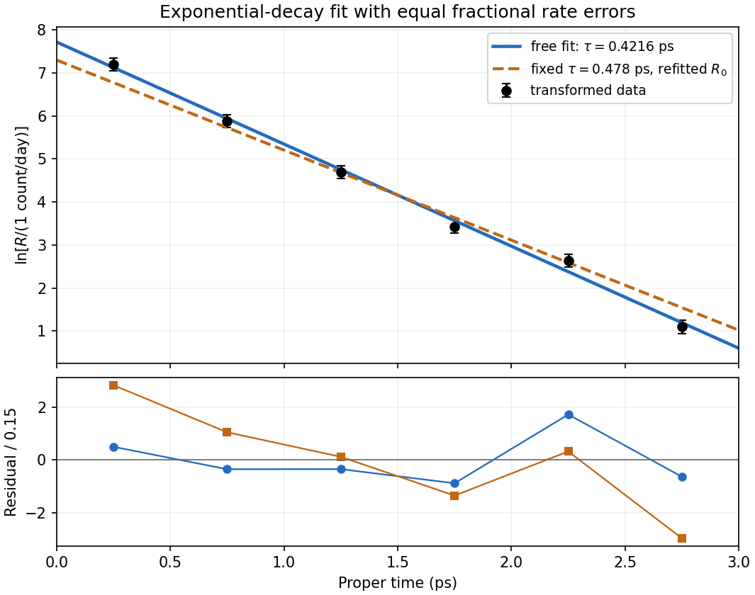
Log-rate fit and the effect of imposing the alternative lifetime
. Original calculation from the exam measurements. The solid line fits both lifetime and normalization; the dashed line fixes and refits its normalization. The lower panel shows standardized log-rate residuals for the two fits. No error bar is assigned to proper time. Details.
For an independent count with a Poisson distribution, collected for exposure at rate , the expected count is and its standard deviation is . The fractional rate uncertainty is consequentlyA target of requires counts at each proper-time setting. The exposure time for a Poisson rate at fixed fractional precision is therefore , givingSince the settings are acquired independently rather than simultaneously,Nearly three quarters of the exposure is spent at the latest, lowest-rate setting. Proper time in picoseconds labels the decay distribution; it is not the laboratory acquisition time in days. This estimate assumes counting statistics dominate, with no additional background-subtraction uncertainty or acquisition overhead.
A chi-squared test compares the sum of squared standardized regression residuals with the appropriate chi-squared distribution. With both line parameters fitted, the data give on degrees of freedom, with upper-tail P-value about : the fitted exponential decay model describes the data adequately.
First consider fixing the alternative lifetime at its central value . Its slope is . One must refit the normalization rather than retain the earlier intercept. Minimization over the intercept gives , andon degrees of freedom, with upper-tail P-value about . Thus that fixed central lifetime gives a substantially worse fit than . Equivalently, the increase after profiling over the intercept isThis fixed-value comparison does not yet include the uncertainty of the alternative measurement.
For the compatibility of independent lifetime measurements, include both errors. Under the approximately Gaussian lifetime-error model, equality of the two true lifetimes is tested byThis has one degree of freedom and P-value approximately , equivalent to a -standard deviation discrepancy. The two measurements are therefore in mild tension: equality is rejected at a significance threshold, but not at . There is no unique yes-or-no compatibility verdict without choosing such a threshold. Treating the alternative central value as exact would overstate the disagreement between the experiments.
The lifetime that provides the best fit to these six rates remains , not . The compatibility calculation above assumes the two experiments have independent uncertainties; a shared systematic error would require its covariance.
Articles by others on the same topic
There are currently no matching articles.