The Born rule gives the required probability by integrating the probability density over the central interval. Put . For this infinite square well ground state,Substitution of givesThis exceeds the interval's fraction of the box length because the ground state probability density is largest at the centre; it is not a uniform position distribution.
Inside the rectangular potential barrier, the electron's wavefunction is evanescent, with decay constantFor width , the squared exponential suppression in the quantum tunnelling probability isThis is the usual leading-exponential estimate. The rectangular-barrier tunnelling probability, retaining the interface-matching prefactor for equal potentials on the two sides, isHere that prefactor is , so the more accurate result is . Both estimates show that transmission is of order one part in a million. A classical particle with this kinetic energy cannot cross the barrier at all.
A Stern-Gerlach experiment sends a collimated beam through an inhomogeneous magnetic field and then measures its transverse position after a drift region. The neutron is electrically neutral but has a nonzero magnetic moment proportional to its spin, . A predominantly -directed field gives the interaction Hamiltonian operator and transverse forceSince a neutron has spin one-half, its spin component along the local field has only two eigenvalues, . Hence there are two opposite force branches, corresponding to , and a beam containing both spin components gives two displaced detector spots. This is neutron Stern-Gerlach splitting, not an electric-charge Lorentz force. A uniform magnetic field can cause Larmor precession but does not provide the required separating magnetic field gradient.
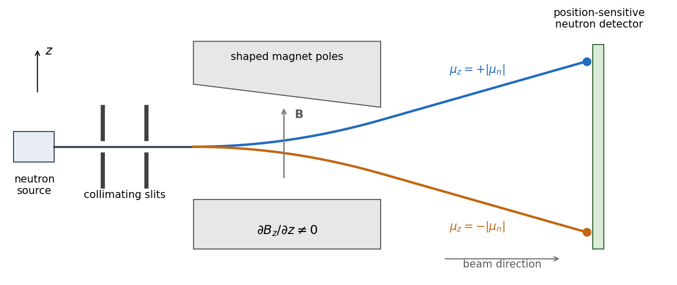

The neutron's gyromagnetic ratio is negative, so its magnetic moment points opposite to its spin; this reverses which spin label goes to which spot without changing the two-way splitting. Equal populations occur for an initially unpolarized beam. A beam prepared entirely in one field-axis spin eigenstate gives only its corresponding branch, explaining the qualification “in general”.
Assume independent background events at a known constant rate, so the background count follows a Poisson distribution. In five months its mean is . The null hypothesis of background alone assigns the observed upward fluctuation the P-valueThusThe tail includes counts above eight because they would be at least as discrepant with the background-only prediction. Even the probability of exactly eight, , exceeds the specified threshold, though it is not the appropriate tail test. The Poisson tail discovery probability is a probability of data under a background model; it is not a posterior probability that the background model is true. This interprets the question's discovery rule in its usual statistical significance sense.
For a real signal with highest frequency , the Nyquist–Shannon sampling theorem gives the nominal Nyquist sampling rateTo cover an arbitrary component exactly at the band edge, choose : a sine sampled at exactly can have every sample equal to zero for an unfortunate phase. Practical aliasing suppression also calls for a margin above the nominal limiting rate.
With rounding to the nearest digitizer level, quantization with step has the uniform-quantization error boundThus the stated digitizer meets the requested nominal amplitude precision per sample, assuming no clipping or other errors. The bandwidth sets the nominal minimum sampling rate; the level spacing sets the rounding precision. Strictly, the sampling theorem reconstructs exactly from exact samples. A uniform error bound on the entire reconstructed continuous waveform is not guaranteed by the level spacing and sampling rate alone; that stronger requirement needs a specified reconstruction and noise model.
The total angular momentum operator is . Since orbital and spin operators act on different factors of the tensor product, they commute, and expanding givesA coupled angular momentum eigenstate is a simultaneous eigenstate of these three squared operators, with eigenvalues , and . Thus the angular factor in the spin-orbit interaction is the numberThe other factor, , is radial. It commutes with the angular operators, and a central-potential energy eigenstate separates into a radial wavefunction and an angular spinor. Taking its radial expectation value therefore givesThis spin-orbit energy shift in a central potential is independent of , so rotational symmetry preserves the magnetic degeneracy within a fixed multiplet. It is a first-order fine structure correction; the given coefficient already includes the relativistic factor needed for the electron's spin-orbit coupling.
The attractive Coulomb potential energy is , soUse precisely the radial normalization stated in the PDF: the radial probability measure is . The supplied function hasIts integral is one, since . In particular,This calculation uses the supplied convention, rather than multiplying a separately normalized standard radial function by an extra .
The addition of angular momentum bracket is . Substitution in the spin-orbit energy shift in a central potential therefore givesHere is the supplied Bohr radius. The negative sign means the member of the pair is shifted downward by this spin-orbit interaction; it is not the total hydrogen binding energy.
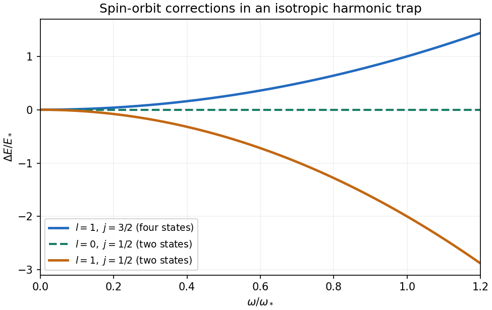
For the isotropic three-dimensional quantum harmonic oscillator, , hence is constant. No radial integral remains, so the spin-orbit energy shift in a central potential reduces toFor , the only possibility is , and the bracket vanishes. For , coupling to spin one-half permits and , whose brackets are and . ThusThese spin-orbit shifts of an isotropic harmonic oscillator are a zero line, a downward parabola, and an upward parabola of half the downward magnitude. They are independent of the radial excitation number, and their magnetic multiplicities are respectively two, two and four. Their weighted mean within the manifold is zero: .

Write and . Inverting the annihilation operator and creation operator definitions givesThe ladder operators take to orthogonal quantum harmonic oscillator energy eigenstates and . Thus , andFor , the lowering term is simply zero. The conclusion concerns an individual energy eigenstate; interference between different eigenstates can produce nonzero expectation values.
For the harmonic-oscillator number-state second moments, the number operator gives , while the canonical commutation relation gives . Terms with or have zero diagonal matrix elements, since they change the occupation number by two. ThereforeConsequently the potential energy and kinetic energy means areTheir sum is the oscillator energy eigenvalue . Their equality is also the virial theorem result for a quadratic potential, here derived directly from the ladder operators.
The standard deviations defining the position and momentum uncertainties satisfy and . Part (a) makes both means zero. Using the second moments from part (b),Multiplication givesThe Heisenberg uncertainty relation requires only . Among the oscillator energy eigenstates, equality occurs solely for the ground state ; the excited states have larger uncertainty products.
Each energy eigenstate picks up its own phase under unitary time evolution. The relative phase therefore changes at . After removing an irrelevant global phase, the state isThe diagonal position matrix elements vanish, but the annihilation operator and creation operator giveThe two off-diagonal cross terms in the expectation value yieldThus the angular frequency is , and the magnitude of the oscillation, meaning its amplitude, isThe peak-to-peak displacement is . The phase fixes where the oscillation starts but does not change . A pure or preparation has no mean oscillation, whereas an equal-weight quantum superposition maximizes its amplitude within this two-state family. The motion is produced by interference between energy eigenstates, rather than by a changing occupation of either one.
Take the natural logarithm of the exponential decay model. To keep the logarithm dimensionless, choose the reference rate and defineThen . With time measured in picoseconds, the slope has units and the intercept is dimensionless. A straight-line linear regression in these variables therefore estimates the inverse mean lifetime and logarithmic normalization.
Use in picoseconds and . Since the time uncertainty is negligible, only the vertical errors enter. First-order propagation of uncertainty givesThe transformed measurements areThus the logarithmic transformation converts constant fractional rate uncertainties into approximately equal absolute log-rate uncertainties. The equality is the linear error approximation; finite error bars would become slightly asymmetric under an exact logarithm.
Assume independent approximately Gaussian log-rate errors with known common standard deviation . The weighted least squares objective isSince all weights agree, the normal equations for linear least squares reduce toFor these data, , , and . Hence and .
The covariance matrix of the fitted slope and intercept follows from the inverse weighted design matrix product, or directly by writing both estimates as linear combinations of the independent :This givesThe parameter conversion and first-order propagation of uncertainty areConsequently,These are one-standard deviation errors. The estimates are correlated, since . The minimum is for four residual degrees of freedom. Because is supplied as a known measurement uncertainty, it should not be rescaled by the observed reduced . This is a log-linear exponential-decay fit.
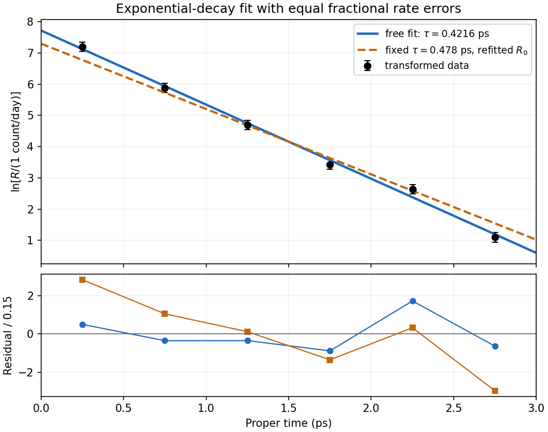
Log-rate fit and the effect of imposing the alternative lifetime
. Original calculation from the exam measurements. The solid line fits both lifetime and normalization; the dashed line fixes and refits its normalization. The lower panel shows standardized log-rate residuals for the two fits. No error bar is assigned to proper time. Details.
For an independent count with a Poisson distribution, collected for exposure at rate , the expected count is and its standard deviation is . The fractional rate uncertainty is consequentlyA target of requires counts at each proper-time setting. The exposure time for a Poisson rate at fixed fractional precision is therefore , givingSince the settings are acquired independently rather than simultaneously,Nearly three quarters of the exposure is spent at the latest, lowest-rate setting. Proper time in picoseconds labels the decay distribution; it is not the laboratory acquisition time in days. This estimate assumes counting statistics dominate, with no additional background-subtraction uncertainty or acquisition overhead.
A chi-squared test compares the sum of squared standardized regression residuals with the appropriate chi-squared distribution. With both line parameters fitted, the data give on degrees of freedom, with upper-tail P-value about : the fitted exponential decay model describes the data adequately.
First consider fixing the alternative lifetime at its central value . Its slope is . One must refit the normalization rather than retain the earlier intercept. Minimization over the intercept gives , andon degrees of freedom, with upper-tail P-value about . Thus that fixed central lifetime gives a substantially worse fit than . Equivalently, the increase after profiling over the intercept isThis fixed-value comparison does not yet include the uncertainty of the alternative measurement.
For the compatibility of independent lifetime measurements, include both errors. Under the approximately Gaussian lifetime-error model, equality of the two true lifetimes is tested byThis has one degree of freedom and P-value approximately , equivalent to a -standard deviation discrepancy. The two measurements are therefore in mild tension: equality is rejected at a significance threshold, but not at . There is no unique yes-or-no compatibility verdict without choosing such a threshold. Treating the alternative central value as exact would overstate the disagreement between the experiments.
The lifetime that provides the best fit to these six rates remains , not . The compatibility calculation above assumes the two experiments have independent uncertainties; a shared systematic error would require its covariance.
The photoelectric effect, black-body radiation and the Davisson–Germer experiment challenge different parts of a fully classical picture. Classical electromagnetic waves successfully describe propagation, interference and diffraction, while classical particles follow trajectories determined by forces. The difficulty is combining that picture with the observed exchange of energy between radiation and matter, the equilibrium distribution of radiation, and electron scattering. The three experiments expose the roles of discrete energy exchange and coherent matter waves.
In a photoelectric effect experiment, monochromatic light illuminates a metal cathode in vacuum and a second electrode collects emitted Electrons. Varying the collecting voltage measures a photocurrent; reversing it until collection ceases determines the stopping potential. The observations distinguish two controls: at fixed frequency above threshold, increasing light intensity increases the emission rate, whereas the largest emitted kinetic energy is determined mainly by frequency. There is a material-dependent photoelectric threshold frequency, and emission above threshold does not require the long charging-up delay predicted by a simple picture of gradual classical energy accumulation at low intensity.
A classical wave carries continuously distributed energy, with intensity proportional to squared field amplitude. On a fully classical absorption picture, increasing intensity would be expected to increase the energy delivered to an electron, and sufficiently long exposure could accumulate the escape energy even below the observed threshold. It does not naturally produce the measured universal straight-line relation between stopping potential and light frequency. In 1905, Albert Einstein instead treated light-energy transfer as localized quanta. His argument distinguished the fastest escaping Electrons from electrons losing energy before escape.[ref]
On a Heuristic Point of View Concerning the Production and Transformation of Light by Albert Einstein. §8, printed pp. 193–196, energy balance and frequency versus intensity predictions
In the single-photon regime, conservation of energy gives the Einstein photoelectric equationwhere is the surface work function. The photon supplies energy ; the escape cost is paid first, and the remainder sets the upper electron-energy edge. Increasing intensity at fixed frequency increases the number of available photons, so it raises current without raising this edge. Below , one photon cannot pay the escape cost. In an actual measurement, stable surface preparation, suppression of unwanted higher-frequency light, and the photoelectric contact-potential correction are needed to test the slope reliably. Robert Andrews Millikan's experiment used selected mercury spectral lines, freshly exposed metal surfaces and an electrometer to make such a quantitative test.[ref]
A Direct Photoelectric Determination of Planck's h by Robert Andrews Millikan. §§2–4, printed pp. 361–375, apparatus and stopping-potential measurements
The interpretation is for weak single-photon illumination; multiphoton photoemission at sufficiently intense fields is a different regime.Black-body radiation tests equilibrium physics rather than the escape of individual electrons. A small aperture in an isothermal absorbing cavity approximates an ideal blackbody: radiation entering the hole undergoes repeated interactions with the walls, and the equilibrium spectrum depends on temperature rather than wall material. A spectrally resolving detector outside the aperture measures how emitted power varies with frequency or wavelength. Experimentally the spectrum has a finite peak, is strongly suppressed at short wavelengths, shifts toward shorter wavelengths when the cavity is heated, and has integrated emission proportional to .
For a large cavity, the electromagnetic mode density in a box, including two independent transverse polarizations, is per volume per unit frequency. The classical equipartition theorem assigns mean energy to each mode, leading to the Rayleigh-Jeans lawThis agrees at low frequencies but diverges as frequency increases; integrating it over all frequencies gives infinite energy density at any nonzero temperature. This is the ultraviolet catastrophe, a failure of classical equipartition applied to the electromagnetic modes.
Max Planck's essential modification was that energy at a frequency is exchanged in units . In a modern oscillator description, the thermal excitation levels are , . Using the Boltzmann distribution and summing a geometric series givesMultiplying by the mode density yields Planck's law for the spectral energy density,When , expansion of the denominator recovers the classical law. When , the large excitation cost suppresses occupancy exponentially, removing the divergence. Its integral gives the Stefan–Boltzmann law, while its peak gives Wien's displacement law. Thus quantization repairs the spectral shape, total emission and temperature dependence together. The displayed thermal energy excludes the oscillator's temperature-independent zero-point energy.
The Davisson–Germer experiment supplies the complementary evidence that matter cannot always be treated as classical particles with definite scattering trajectories. In 1927, Clinton J. Davisson and Lester Halbert Germer sent a narrow, accelerated electron beam normally onto a single nickel crystal in vacuum. A movable collector measured the current of scattered Electrons as direction and accelerating voltage were varied; a retarding potential selected electrons retaining approximately the incident energy. Sharp angular beams depended on crystal orientation and beam energy, with a prominent feature near and detector colatitude . These are scattering directions and currents, not photographs of electron paths.[ref]
Diffraction of Electrons by a Crystal of Nickel by C. Davisson and L. H. Germer. Printed pp. 707–710, apparatus; pp. 715–719, voltage and angular scans
The de Broglie wavelength predictsAt , this gives , comparable to atomic spacings. A crystalline arrangement supplies regularly spaced scattering sites, so scattered probability amplitudes can add constructively in selected directions. For a suitable family of crystal planes, Bragg's law expresses the condition as , with measured relative to those planes. The detector colatitude is not automatically this angle. The measured angular structure and its variation with electron momentum are described by electron diffraction with the de Broglie wavelength. A classical point-particle deflection model has no phase wavelength and does not supply that interference condition.
The common quantum account preserves the successes of wave propagation and particle detection while changing what is quantized. Photons exchange energy in frequency-dependent units; a thermal distribution of those excitations gives the blackbody spectrum. Electrons have a wavefunction whose amplitudes interfere on scattering from a crystal, while detection transfers localized charge. The Born rule turns squared amplitudes into event probabilities. These results invalidate a fully classical description of matter and radiation; the photoelectric energy law alone does not establish every property of a quantized electromagnetic field, but the three phenomena together provide complementary evidence for the quantum description.
For the deep-water gravity wave, the phase velocity and group velocity follow from its dispersion relation:The wave packet travels at , while the individual crests travel at . Let its effective length be , where is the carrier wavelength. A fixed observer is inside the wave packet for , and crests arrive with wave period . ThusCrests enter the rear of the moving wave packet and disappear at its front, so the five visible at one instant are not five permanently identifiable crests. The count uses the intended narrow-band, approximately unchanged wave packet and neglects the precise visibility of its end crests.
A bubble is a thin water layer surrounded by air. At a locally flat patch, let its thickness be , its refractive index be , and the internal angle of refraction be . The two principal reflected light contributions are the reflection at the first surface and the contribution that enters the layer, reflects at its second surface and leaves again. The first reflection, from lower to higher refractive index, introduces a phase shift; the second does not. Their optical path difference is , so their phase difference is, modulo ,where is the vacuum wavelength. Constructive interference in reflected light therefore occurs approximately whenDestructive interference occurs at . In the weak-reflection approximation, the reflected light intensity at each wavelength is proportional to . This is a smooth spectral filter, with broad maxima and minima: it does not select three pure wavelengths corresponding to display primaries. Ordinary illumination contains many visible wavelengths, and the eye combines their remaining contributions through color vision. The result is a mixture of colours, often pastel or desaturated.
The layer thickness varies over the bubble because of drainage and flow; the bubble's curvature also changes the local angle of refraction and the viewed optical path difference. The spectral filter therefore changes continuously across the surface and in time. Very thin regions become dark because the two reflected contributions nearly cancel across the visible optical spectrum. Thin-film interference explains both the changing colours and this dark limit.
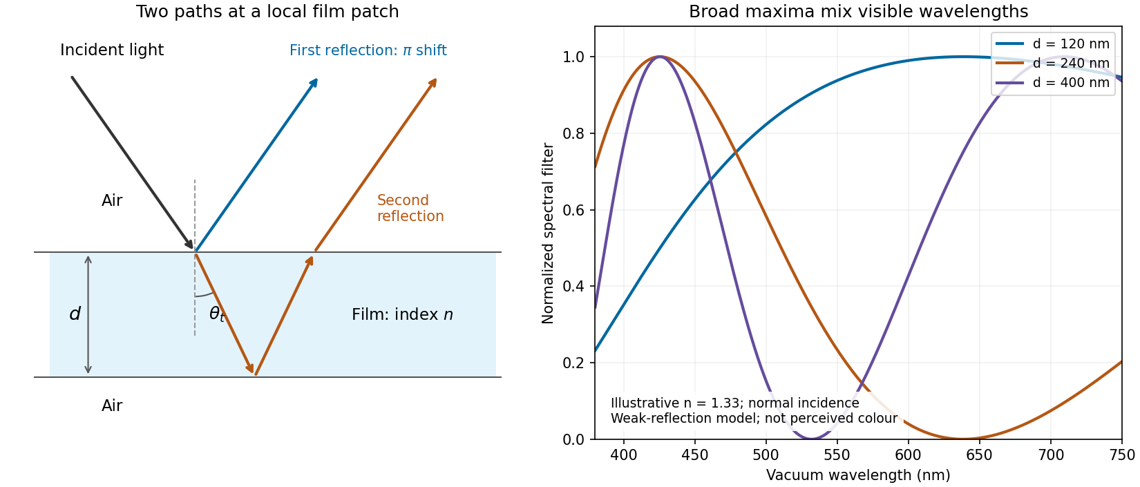
Two reflected paths through a thin film and the broad spectral filtering that produces mixed colours
. Details. 
The ray sketch shows a local patch and is not to scale. The plotted curves use a chosen constant at normal incidence and illustrative thicknesses; they show the spectral filter rather than calibrated perceived colours.
Model the room's decaying acoustic waves as a weakly damped resonator. The quality factor from ringdown is related to stored energy bywhere is the pressure wave amplitude and . The measured frequency gives . If the stated is interpreted as an approximate wave amplitude exponential relaxation time,an estimate of order . Taking as an energy exponential relaxation time instead gives .
There is a real convention ambiguity: “heard to die away” gives neither an initial sound level nor an audibility threshold, so it does not determine either exponential relaxation time. More generally, if the energy falls by a factor in ,In room acoustics, a reverberation time usually denotes a decibel drop of , or an energy factor . If means , the corresponding estimate is instead . The simple decay-time estimate and the conventional reverberation time estimate should not be silently equated.
The three primitive lattice translation vectors join a cube corner to the three adjacent face centres. Thus the Bravais lattice is a face-centered cubic lattice, with conventional cubic side .
Write the given primitive lattice translation vectors as . Their primitive unit cell volume isThe reciprocal lattice convention then givesEach reciprocal lattice vector has units when is in metres. Integer combinations generate a body-centered cubic lattice of conventional cubic side ; the point is its body centre. Directly taking the nine dot products checks the signs and the normalization.
Let be the integer number of primitive unit cells. A Bloch state can be written as , with . The periodic boundary condition therefore requiresThe spacing of allowed wavevectors is . The first Brillouin zone has width , soFor an exact endpoint convention take a half-open Brillouin zone, such as . Its two endpoints differ by a reciprocal lattice vector and must not both be counted as distinct values of crystal momentum. There are exactly inequivalent integers modulo , irrespective of whether is even or odd. This is state counting in a Bloch band: one allowed wavevector per primitive unit cell per energy band. A separate twofold spin multiplicity gives electronic states per energy band, without doubling the number of wavevectors.
Use transverse displacement , small slopes and constant tension . For a short string element of length , Newton's second law gives . Hence the wave equation on a string iswhere is the linear mass density, in .
The mechanical impedance of a rightgoing travelling wave is the transverse driving force divided by the transverse velocity at the driven section. Choose the force exerted by the material to the left on the material to the right, . For , the transverse velocity is . Thus the positive characteristic impedance of a stretched string isA leftgoing component has with this fixed orientation of force. Specifying the orientation avoids confusing that propagation sign with a negative material mechanical impedance.
Place the junction at and use the complex amplitude convention . With incident displacement wave amplitude , writeHere and are displacement wave reflection and transmission coefficients, and . The junction is assumed massless, with no externally applied transverse force, and both strings have the common equilibrium tension . Continuity of displacement and transverse force givesSince , these become and . Solving,A larger right-hand mechanical impedance produces a reflected displacement with reversed sign, as expected in the fixed-end limit . Equal mechanical impedances give and .
The instantaneous rightward energy flux along a string is the transverse force times the transverse velocity,For a rightgoing time-harmonic wave of peak displacement wave amplitude , averaging over a wave period givesA leftgoing time-harmonic wave has the opposite signed energy flux. The positive ratios of reflected and transmitted power to incident power are thereforeAll explicit angular frequency factors cancel. In the ideal wave equation on a string, and the two linear mass densities are constant, so the mechanical impedances have no frequency or wavelength dependence. Consequently is independent of wavelength even though the two string wavelengths generally differ.
Finally,This is conservation of energy at a lossless, massless junction. The transmitted displacement wave amplitude can exceed the incident one when ; the factor is essential when comparing power.
Let the middle segment occupy . Normalize the incident displacement complex amplitude to one, suppress the common time factor , and chooseHere is the reflected complex amplitude at , and are the rightgoing and leftgoing middle-segment complex amplitudes referenced to , and is the outgoing complex amplitude referenced to . The middle wavenumber is , andis the propagation phase factor across the lossless middle segment.
At each junction, continuity of displacement and transverse force means continuity of and . Using givesThese boundary conditions also include all multiple reflections inside the middle segment: and are the total travelling components, not just the first waves to cross a junction.
Put . Eliminating the middle-segment complex amplitudes using the right-hand boundary conditions givesHence the displacement reflection coefficient isFor finite positive real mechanical impedances, its denominator cannot vanish at real . The real and imaginary parts of the numerator must therefore vanish separately:This gives all three possibilities.
If the exterior strings differ, , then , so andThe middle segment is a quarter-wave impedance transformer. Its two reflected contributions cancel at these odd quarter-wavelength thicknesses. Here is specifically the wavelength in the middle string; the matching is not generally valid at every frequency.
If but differs, the second condition requires , givingA whole number of half-wavelengths reproduces the exterior mechanical impedance at the input. The formal limit is zero frequency or zero segment length, rather than a finite-wavelength resonance.
Finally, if , both conditions hold identically: . Since the system is lossless, each of these cases also gives unit transmitted power.
The expression is a scalar diffraction theory integral for a monochromatic wave. The complex quantity represents a field complex amplitude, with physical field obtained by taking the real part after multiplication by . The light intensity is proportional to . The coordinates label transverse positions in the aperture plane, is its transmitting region, and is the incident field multiplied by the aperture's complex transmission. The wavenumber is in the propagation medium, and is the axial propagation distance if already includes the incident field.
To derive the Fresnel diffraction, start from Huygens-Fresnel principle contributions with propagation factor . With the coordinate origin at the projection of into the aperture plane,The paraxial approximation requires , where . Replace the slowly varying and the obliquity factor by their axial values, but retain the quadratic variation of wave phase. Neglect of the next wave phase term requires over the relevant aperture. Thus, apart from a common constant,The quadratic wave phase may be of order one or much larger; setting it to zero would require the stronger conditions for Fraunhofer diffraction. The scalar treatment also neglects the detailed vector field at aperture edges and assumes dimensions large enough compared with wavelength for this approximation to be useful.
For a finite-distance axial point source at distance and an observer at distance , the incident field contributes its own quadratic wave phase. If instead denotes only the aperture transmission, the combined curvature is described by an effective distanceThese are two equivalent conventions for distributing the incident wave phase between and the exponential. Both distances must be included in the later calculation.
Write and for the axial source and observation distances, and put . The aperture is . Under the Fresnel diffraction, the spherical incident wave amplitude is effectively constant over this small aperture, while its quadratic wave phase must be retained. Therefore the two transverse integrals separate:where contains the source strength, the propagation distances and a common phase factor.
Use the dimensionless variable and define the optical normalization of Fresnel integralsThe oddness of makes the bracket , soThis square-aperture Fresnel diffraction normalization is especially useful for comparing with no aperture. In the same Fresnel diffraction, the unrestricted one-dimensional Fresnel integral is ; its square is . Thus, writing for the unobscured field at the same point,The normalization has the correct no-aperture limit because in this convention.
Use SI units throughout: , , and . The effective propagation distance is , givingIn the supplied Cornu spiral, the endpoint at is approximately . HenceMore accurate Fresnel integrals, and , give . The central light intensity is increased to about times the unobscured value, an increase of roughly .
There is no violation of conservation of energy: the aperture reduces the total transmitted power, while removing contributions that partly cancel the central field redistributes the transmitted power across the observation plane. In particular, the square aperture does not give the same central field as a circular aperture of a superficially similar size.
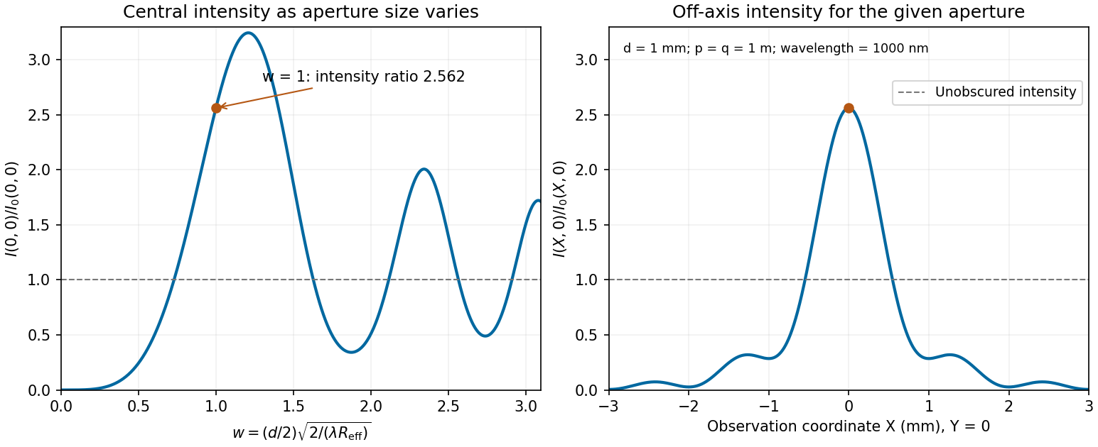
Calculated central intensity and an off-axis section for the square aperture in the Fresnel approximation
. Details. 
Let the source remain at and let the observation point be . The paraxial approximation to the source-to-aperture-to-observer optical path length isCompleting the squares givesThe point is where the straight source-observer line intersects the aperture. Define the four dimensionless edge positionsOn the Cornu spiral , draw the directed chord from to , and a second directed chord from to . Denote their complex differences by and . The complex amplitude is proportional to their product: multiply their lengths and add their arguments, including the common propagation phase factor.
More explicitly, normalize by the unobscured field at this same observation point. The constant wave phase from completing the square is then already included in , andEach directed chord is a one-dimensional Fresnel diffraction factor. One must multiply the two factors, rather than add the chords or use just one chord length for the square aperture. Setting recovers and the on-axis answer.
The crystal has periodic potential . By Bloch's theorem, an energy eigenstate may be chosen asExpand the periodic factor in a Fourier series:Multiplication by gives the stated plane-wave expansion. Here is position, is the primitive unit cell length, is the primitive reciprocal lattice wavenumber, runs over every integer, and are complex numbers specifying the component wave amplitudes. The wavevector labels the Bloch state modulo ; is its crystal momentum, rather than generally its measured free-space momentum.
The component is a plane wave of wavevector . All these components acquire the same phase factor under , since . Their mixing therefore respects the crystal's translation symmetry. The coefficients and energy eigenvalue follow from the Schrödinger equation; the expression is not a claim that the coefficients are equal or that only finitely many are nonzero. The energy band index is suppressed in the notation, so different energy bands at a common generally have different coefficient sets.
Choose the Fourier series conventionFor a real potential energy, . The symbol means the Fourier coefficient , with units of energy, rather than the pointwise value of at a position .
Retain the two plane waves and in the nearly-free electron model. Their kinetic energies are and . The matrix representation of a linear map for the Quantum Hamiltonian projected onto this two-dimensional basis isThus givesSolving this quadratic equation yieldsChoosing the zero of potential energy so that its spatial average is reproduces the requested expression. If that average has not been removed, both energy bands are shifted by ; no band gap, group velocity or effective mass is changed by this constant shift.
The two kinetic energies coincide at . Their coupling gives an avoided crossing with band gap . The result is exact within the projected two-wave Quantum Hamiltonian. It is an approximation to the full crystal problem, appropriate near this crossing for a weak periodic potential whose other Fourier coefficients do not cause strong mixing with remote plane waves. Small alone would not justify ignoring arbitrarily large other Fourier coefficients.
Set , , and . The two kinetic energies satisfyConsequently the nearly-free electron dispersion near a one-dimensional band gap becomesThe Taylor expansion givesFor the paper's energy convention, set . There is no linear or cubic term because each branch is an even function of displacement from the crossing in this two-wave approximation. Each coefficient multiplying has units of energy times length squared, as required.
The expansion requiresa more restrictive condition than merely when the band gap is small. If , the square root is proportional to and this analytic expansion of the energy-ordered branches is unavailable.
Twice the quadratic coefficient from the previous part is the band curvature . Thus the band effective masses areHere and . In the weak-potential regime ,Both have units of mass; their magnitudes are much smaller than in this asymptotic regime. The upper energy band has a local minimum and positive effective mass, while the lower energy band has a local maximum and negative effective mass. The exact lower-branch sign changes at in the two-wave formula; the intended weak-coupling limit lies below that threshold.
The physical meaning follows from the semiclassical equations for an Electron wave packet in one energy band:An upper-band Electron near its minimum accelerates in the direction of the applied force, whereas a lower-band Electron near its maximum accelerates opposite to it. At the extremum itself the group velocity is zero. A nearly filled lower energy band is conveniently described by electron holes with positive electric charge and positive effective mass . Negative curvature is a response of a crystal energy eigenstate, not a negative bare electron mass. These statements assume slow forcing that does not induce transitions across the band gap.
In a metal, a partially filled energy band or overlapping energy bands supplies Electrons with nearby unoccupied states. At thermal equilibrium, oppositely directed group velocities are equally populated and the net electric current vanishes. An applied electric field distorts the occupation distribution, producing a small mean drift velocity. A filled energy band alone has no such low-field intraband response because its velocity contributions cancel over the entire Brillouin zone.
In the Drude model, let be the mobile Electron number density, let be the elementary charge, and let be the momentum relaxation time. The mean motion obeysThe steady state is . The current density is opposite to the Electron drift velocity:This gives microscopic Ohm's law, with electrical conductivity in and electrical resistivity in . For a uniform wire of length and cross-sectional area , its electrical resistance is . The dissipated power per volume is , the Joule heating supplied by the external source.
The free electron model with Fermi-Dirac statistics improves the microscopic picture. The Pauli exclusion principle fills states up to the Fermi energy at low temperature. For a spherical, parabolic energy band with two spin states,Only states near the Fermi surface change their occupation in a weak-field response; the large equilibrium Fermi velocity is not the small drift velocity. The same formula results for this isotropic parabolic model when is evaluated for transport near the Fermi surface. In a crystal, the energy band group velocity, effective mass and possibly direction-dependent scattering replace the simplest bare-particle picture. The mean free path is approximately .
A perfectly periodic static lattice is already included in Bloch states and does not by itself give a finite electrical resistivity. Momentum relaxation comes from defects, impurities, boundaries, and electron-phonon scattering. Independent scattering mechanisms approximately add their rates, giving Matthiessen's rule,The approximately temperature-independent is the residual resistivity. In ordinary simple metals, the phonon contribution is approximately proportional to temperature at high temperature; a three-dimensional acoustic-phonon transport model gives a contribution well below the relevant Debye temperature. Other mechanisms can dominate in particular materials or regimes, so neither power law is universal.
The classical Drude model incorrectly treats the equilibrium carrier statistics. Fermi-Dirac statistics explains the small electronic heat capacity, while electrons carrying both charge and heat give the approximate Wiedemann-Franz law for degenerate carriers with appropriate nearly elastic scattering. Both the simple electrical conductivity formula and this thermal relation depend on the assumptions about energy bands and scattering, rather than being exact for all metals.
The Debye model approximates a three-dimensional crystal as an elastic continuum supporting quantized normal modes, or phonons. At long wavelengths, the acoustic phonon branches have approximately linear dispersion relations : one longitudinal branch and two transverse branches. Replace their complicated actual spectra by these linear forms, then introduce a cutoff chosen to preserve the total vibrational degrees of freedom for atoms. This is an approximation to the spectrum, not a claim that a real crystal has no non-acoustic branches.
For periodic boundary conditions in volume , each allowed wavevector occupies in the space of wavevectors. Counting a spherical shell for each branch gives the density of states per unit angular frequencyAn effective speed of sound can be defined by . In the single-speed Debye model, choose so thatThus the Debye wavevector, Debye frequency and Debye temperature satisfyHere has units of seconds when angular frequency is measured in ; its integral is the dimensionless number of normal modes. The spherical cutoff replaces the real Brillouin zone by an equal-count continuum construction.
Each phonon mode is a quantum harmonic oscillator. Since phonon number is not conserved at thermal equilibrium, the chemical potential is zero and its Bose-Einstein distribution gives mean thermal energy . The zero-point energy is independent of temperature in the harmonic, fixed-volume approximation and does not contribute to the heat capacity at constant volume. Excluding that constant term,Differentiating the first integral at fixed volume avoids losing the temperature-dependent upper limit in the second one. The resulting Debye heat capacity isFor , extend the upper limit to infinity. Expanding and integrating term by term gives . ThereforeThis law follows from the three-dimensional density of states and the availability only of low-frequency modes at low temperature. It is a central success of the Debye model.
For , the Bose-Einstein distribution reduces to the classical equipartition theorem: every mode contributes thermal energy . Consequentlythe Dulong-Petit law, or per mole of atoms. The simple model omits detailed phonon dispersion relation, distinct optical phonon branches, and anharmonic effects such as thermal expansion. In a metal, the low-temperature total heat capacity additionally contains a term approximately proportional to from Electrons, so the lattice term should not be mistaken for the whole measurement.
Articles by others on the same topic
There are currently no matching articles.