The boundary-value method. In a charge-free region, the electric potential obeys the Laplace equation, , and . Conductors impose equipotential boundaries, with specified voltages or charges, and a far-field condition fixes the remaining behaviour. The Uniqueness of the Dirichlet problem guarantees that a solution meeting the prescribed conductor potentials is the physical one. To see why, the difference of two candidate solutions is harmonic and vanishes on the boundaries; integration by parts gives , hence no difference in their fields. An exterior problem also needs the appropriate condition at infinity.
Two axisymmetric harmonic functions. For in spherical coordinates, the Laplacian reduces toFor , the bracket is . For , it is . ThereforeThe second function is singular at the origin, which is allowed here because that point lies inside the excluded conductor. The printed spherical Laplacian has a typo in its azimuthal term: its denominator should be . Both functions are axisymmetric, so that term vanishes and the typo does not affect these calculations.
Potential and field geometry. Set the lower conductor to zero potential and the distant upper plate to . The small boss sees approximately uniform background field , where . Combining the two harmonic functions to make on gives the conducting hemispherical protrusion in a uniform field,It also vanishes on the surrounding plane . The electric field components areEquipotentials crowd near the apex, and field lines meet the conductor normally.
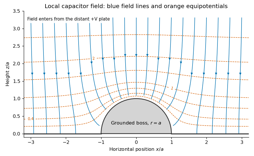
Original calculated local equipotentials and electric-field lines above the hemispherical boss; this is the small-boss approximation rather than an exact finite-gap solution
. Details. 
The formula has the correct uniform far field but does not exactly impose a flat upper equipotential at finite . It is the leading approximation justified by ; an exact finite-gap solution would include further corrections.
Articles by others on the same topic
There are currently no matching articles.