The boundary-value method. In a charge-free region, the electric potential obeys the Laplace equation, , and . Conductors impose equipotential boundaries, with specified voltages or charges, and a far-field condition fixes the remaining behaviour. The Uniqueness of the Dirichlet problem guarantees that a solution meeting the prescribed conductor potentials is the physical one. To see why, the difference of two candidate solutions is harmonic and vanishes on the boundaries; integration by parts gives , hence no difference in their fields. An exterior problem also needs the appropriate condition at infinity.
Two axisymmetric harmonic functions. For in spherical coordinates, the Laplacian reduces toFor , the bracket is . For , it is . ThereforeThe second function is singular at the origin, which is allowed here because that point lies inside the excluded conductor. The printed spherical Laplacian has a typo in its azimuthal term: its denominator should be . Both functions are axisymmetric, so that term vanishes and the typo does not affect these calculations.
Potential and field geometry. Set the lower conductor to zero potential and the distant upper plate to . The small boss sees approximately uniform background field , where . Combining the two harmonic functions to make on gives the conducting hemispherical protrusion in a uniform field,It also vanishes on the surrounding plane . The electric field components areEquipotentials crowd near the apex, and field lines meet the conductor normally.
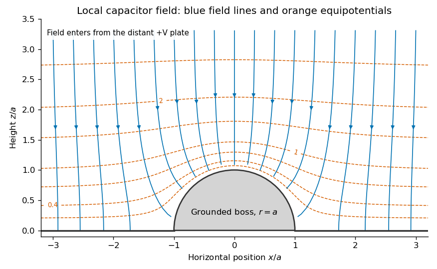
Original calculated local equipotentials and electric-field lines above the hemispherical boss; this is the small-boss approximation rather than an exact finite-gap solution
. Details. 
The formula has the correct uniform far field but does not exactly impose a flat upper equipotential at finite . It is the leading approximation justified by ; an exact finite-gap solution would include further corrections.
At the hemispherical surface , the outward normal from the conductor into the gap is . The tangential field is zero there andThe electrostatic interface boundary conditions give surface charge density , because the interior electric field is zero. HenceIt is negative for a positive upper-plate voltage, greatest in magnitude at the apex, and zero at the equator. Its units are coulombs per square metre.
On the lower plane outside the boss, write for distance from the boss centre along the plane, so . Differentiate the potential normally before putting :Thus the normal field is andThe source uses for this distance on the plane. Near the rim it tends to zero, while far from the boss it recovers the uniform parallel-plate surface charge.
The largest gap field is at the apex: . If the fixed breakdown threshold is , a smooth parallel-plate gap permits , whereas this small hemispherical boss permitsThus the maximum voltage is reduced by a factor of three, within the stated local-field approximation. This comparison holds the material dielectric strength and gap fixed.
The field law. In the Biot-Savart law, is the contribution to the magnetic flux density at the observation point from a directed wire element carrying steady conventional electric current . The vector points from that element to the observation point, , and . The constant is the vacuum permeability; the cross product sets the direction by the right-hand rule. Integrating the elements gives the total field, in teslas.
The moment of the shown loop. The arrows in the original PDF run counterclockwise viewed from . Thus the magnetic dipole moment isIts units are . Reversing the current reverses both this moment and the field.
Use source coordinates and observation point . The axial numerator in the Biot-Savart law isFor much larger than the loop dimensions, replace the denominator by to leading order. Transverse components cancel between opposite sides. The loop integral is twice its oriented area, soThereforeIt points along on both halves of the dipole axis, not along the signed radial unit vector.
At the field is perpendicular to the loop plane. Its Biot-Savart numerator isThe leading denominator variation must be kept:The integral of is zero, but its product with is not. Keeping all terms of the leading nonzero order givesFor the counterclockwise rectangle, and . HenceThis transverse field is opposite to the magnetic dipole moment. Replacing every denominator by a constant before examining the term proportional to would give the wrong answer.
Why the shape is immaterial far away. Partition an arbitrary small planar loop into small rectangular loops with the same oriented current. Currents on internal shared edges cancel, leaving only the original boundary. Their magnetic dipole moments add to , with the enclosed area. Far enough away, the leading fields add as dipoles at the same position. The general magnetic dipole field isHigher spatial multipoles contain shape-dependent corrections. The axial and transverse results above are the special directions of this expression.
The aligned terrestrial model. Take the moment to point toward geographic south. At northern latitude , the magnetic dipole inclination versus latitude gives local northward and downward componentsUsing the specified and ,The direction is geographic north and below horizontal, with no eastward component in this ideal model. These values use the latitude printed in the paper.
Effective permittivity. Use peak phasors with time dependence . The Ampere-Maxwell law isThe conductive contribution to complex permittivity is thereforeHere is the source's effective relative permittivity, not just the real part of a complex response. The positive imaginary term is the loss sign appropriate to this time convention.
The penetrating electric wave. Combine this equation with Faraday's law of induction. In a uniform source-free medium the transverse phasor satisfiesFor a good conductor of electrical conductivity , , so . The root which decays into isChoose the surface phasor amplitude real. Taking the real part of givesThe skin depth is an amplitude-decay distance in metres.
The magnetic wave and phase. The curl of an -polarized field varying in is in the direction. Since ,ThusThe phase sign follows the specified convention. Equivalently the surface impedance of a good conductor is .
How the fields differ from those in vacuum. The two metal fields have the same exponential envelope and spatial period , but their phase arguments differ by .
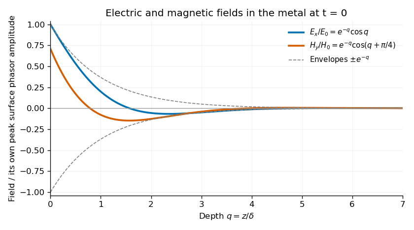
Original normalized electric and magnetic field profiles inside a good conductor at one instant, showing their common decay envelope and quarter-of-a-right-angle phase difference
. Details. 
An individual travelling wave in the lossless exterior has no attenuation, real wave impedance and in-phase electric and magnetic fields. The exterior total field also includes the reflected wave and may show interference, so it need not share that simple phase relation everywhere. At the interface the tangential fields match; is the field just inside the metal, not necessarily the incident amplitude. A good conductor reflects strongly and its wave impedance is much smaller than the vacuum impedance.
Average inward energy flux. For peak phasors, the Poynting vector averaged over a cycle is . The fields giveConsequently the constant in the question isThe flux is in the direction and has units .
Local energy conservation. The Poynting flux and local heating in a skin layer satisfyThe decrease becomes Joule heating in each layer. The Poynting theorem includes this transfer from field energy to the metal; averaged electromagnetic energy storage has zero time derivative in the periodic state, so no energy is lost from the complete balance.
Distributed line parameters. The geometry is the wide parallel-plate transmission line described in the question, with absolute permittivity . A length has charge and field , givingThe opposed plate currents have sheet density and confine the leading magnetic field between the plates. The magnetic energy per unit length is , soHere and are per unit length, in and , not lumped component values. Internal conductor fields and edge corrections are neglected.
Voltage and current evolution. The current entering a short length minus that leaving it is the rate of increase of its plate charge:The voltage drop across that length is its inductive drop, . Dividing by gives the lossless Telegrapher's equations,
Propagation speed. Differentiate these equations once more and eliminate the other variable:The wave equation speed is
Travelling-wave impedance. For a forward wave , take . Substitution into gives , hence the characteristic impedanceThe backward-wave current has the opposite sign relative to its voltage; the fixed ratio above applies to one travelling direction.
Matching the antenna. The voltage reflection coefficient is . No reflection requires . With , , and ,The resulting is consistent with the wide-plate approximation.
Both transverse forces. The matched transverse electromagnetic mode has electric attraction and magnetic repulsion. For time-averaged power ,The force on one plate excludes its own field. Thus the average electric attraction and magnetic repulsion per unit length are respectivelyThe electric and magnetic pressure cancellation in a matched TEM line follows directly from :The equality also holds instantaneously for a single travelling wave. Quoting either alone would omit the opposing contribution. This is the ideal electromagnetic force in the stated lossless uniform-dielectric model; a standing wave would not generally have the same cancellation.
Articles by others on the same topic
There are currently no matching articles.