An infinite sheet of surface charge density gives an electric field of magnitude on either side, normal to the sheet and directed away from positive charge. Use the superposition principle for the two sheets. Choose normals for and for . Away from the charged planes,The minus sign on the second contribution makes its field point toward the negatively charged sheet. Each sector has a uniform electric field; its direction changes on crossing a sheet.
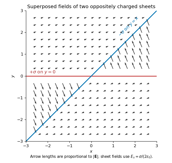
Original calculated electric-field directions for the intersecting positive and negative charge sheets; arrows retain the relative field magnitudes in the four sectors
. Details. 
For example, above both sheets the field points right and slightly upward, whereas in the sector but it points left and steeply upward. The other two sectors follow by inversion through the origin. The normal field jumps by the appropriate surface charge divided by ; a single field value on an ideal zero-thickness charged sheet is not required.
Let the signed axial velocity on the axis be . Smooth axisymmetric flow has and regular radial velocity at . The incompressible flow condition in cylindrical coordinates isTo leading order near the axis, integrate from zero to . The integration constant vanishes by regularity, giving the near-axis radial velocity in incompressible axisymmetric flow,With the usual signed interpretation ,For this is outward: the outward axial flow slows as its distance from the origin grows, and incompressibility requires radial spreading. Here has units , so the answer is a speed.
The source specifies a magnitude rather than an unambiguous signed component. On , reversing the axial flow while keeping its magnitude would reverse the radial answer. The general relation makes that dependence explicit; the boxed expression adopts , outward on both halves of the axis.
A large gas volume can reduce the effective mass density of the water surrounding the hull. In the simple quasihydrostatic model for the buoyancy of an aerated liquid, gas void fraction givesBy Archimedes' principle, a boat displacing volume then has buoyant force . To support the same boat mass , it needs a larger displaced volume , so its draft increases. If that exceeds the available watertight displacement, it can lose flotation or become swamped:Uneven aeration and strong plume motion can also disturb stability. This explains a possible hazard, not a claim that any bubble plume must sink a boat: upward water flow, turbulence and the distribution of bubbles can exert substantial additional forces.
The conventional electron plasma frequency isUse , , and . ThenThe equal proton density ensures charge neutrality; it does not double the electron density in this formula. Protons have their own plasma frequency,If both cold species are allowed to move in the relative charge-separation oscillation, its squared frequency is . This gives , only about above the electron-only answer, because .
Apply equal compressive pressure in all directions; here denotes Poisson's ratio. The three principal normal stresses are . For an isotropic linearly elastic material, Hooke's law givesand similarly for . At small strain, the fractional volume change is the sum of these normal strains:The bulk modulus is , giving the isotropic elastic modulus relation,The result assumes linear elasticity and fixed isotropic moduli. In the incompressible limit with finite Young's modulus, the bulk modulus tends to infinity.
The boundary-value method. In a charge-free region, the electric potential obeys the Laplace equation, , and . Conductors impose equipotential boundaries, with specified voltages or charges, and a far-field condition fixes the remaining behaviour. The Uniqueness of the Dirichlet problem guarantees that a solution meeting the prescribed conductor potentials is the physical one. To see why, the difference of two candidate solutions is harmonic and vanishes on the boundaries; integration by parts gives , hence no difference in their fields. An exterior problem also needs the appropriate condition at infinity.
Two axisymmetric harmonic functions. For in spherical coordinates, the Laplacian reduces toFor , the bracket is . For , it is . ThereforeThe second function is singular at the origin, which is allowed here because that point lies inside the excluded conductor. The printed spherical Laplacian has a typo in its azimuthal term: its denominator should be . Both functions are axisymmetric, so that term vanishes and the typo does not affect these calculations.
Potential and field geometry. Set the lower conductor to zero potential and the distant upper plate to . The small boss sees approximately uniform background field , where . Combining the two harmonic functions to make on gives the conducting hemispherical protrusion in a uniform field,It also vanishes on the surrounding plane . The electric field components areEquipotentials crowd near the apex, and field lines meet the conductor normally.
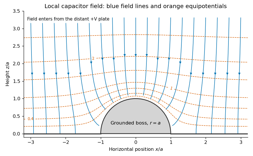
Original calculated local equipotentials and electric-field lines above the hemispherical boss; this is the small-boss approximation rather than an exact finite-gap solution
. Details. 
The formula has the correct uniform far field but does not exactly impose a flat upper equipotential at finite . It is the leading approximation justified by ; an exact finite-gap solution would include further corrections.
At the hemispherical surface , the outward normal from the conductor into the gap is . The tangential field is zero there andThe electrostatic interface boundary conditions give surface charge density , because the interior electric field is zero. HenceIt is negative for a positive upper-plate voltage, greatest in magnitude at the apex, and zero at the equator. Its units are coulombs per square metre.
On the lower plane outside the boss, write for distance from the boss centre along the plane, so . Differentiate the potential normally before putting :Thus the normal field is andThe source uses for this distance on the plane. Near the rim it tends to zero, while far from the boss it recovers the uniform parallel-plate surface charge.
The largest gap field is at the apex: . If the fixed breakdown threshold is , a smooth parallel-plate gap permits , whereas this small hemispherical boss permitsThus the maximum voltage is reduced by a factor of three, within the stated local-field approximation. This comparison holds the material dielectric strength and gap fixed.
The field law. In the Biot-Savart law, is the contribution to the magnetic flux density at the observation point from a directed wire element carrying steady conventional electric current . The vector points from that element to the observation point, , and . The constant is the vacuum permeability; the cross product sets the direction by the right-hand rule. Integrating the elements gives the total field, in teslas.
The moment of the shown loop. The arrows in the original PDF run counterclockwise viewed from . Thus the magnetic dipole moment isIts units are . Reversing the current reverses both this moment and the field.
Use source coordinates and observation point . The axial numerator in the Biot-Savart law isFor much larger than the loop dimensions, replace the denominator by to leading order. Transverse components cancel between opposite sides. The loop integral is twice its oriented area, soThereforeIt points along on both halves of the dipole axis, not along the signed radial unit vector.
At the field is perpendicular to the loop plane. Its Biot-Savart numerator isThe leading denominator variation must be kept:The integral of is zero, but its product with is not. Keeping all terms of the leading nonzero order givesFor the counterclockwise rectangle, and . HenceThis transverse field is opposite to the magnetic dipole moment. Replacing every denominator by a constant before examining the term proportional to would give the wrong answer.
Why the shape is immaterial far away. Partition an arbitrary small planar loop into small rectangular loops with the same oriented current. Currents on internal shared edges cancel, leaving only the original boundary. Their magnetic dipole moments add to , with the enclosed area. Far enough away, the leading fields add as dipoles at the same position. The general magnetic dipole field isHigher spatial multipoles contain shape-dependent corrections. The axial and transverse results above are the special directions of this expression.
The aligned terrestrial model. Take the moment to point toward geographic south. At northern latitude , the magnetic dipole inclination versus latitude gives local northward and downward componentsUsing the specified and ,The direction is geographic north and below horizontal, with no eastward component in this ideal model. These values use the latitude printed in the paper.
Effective permittivity. Use peak phasors with time dependence . The Ampere-Maxwell law isThe conductive contribution to complex permittivity is thereforeHere is the source's effective relative permittivity, not just the real part of a complex response. The positive imaginary term is the loss sign appropriate to this time convention.
The penetrating electric wave. Combine this equation with Faraday's law of induction. In a uniform source-free medium the transverse phasor satisfiesFor a good conductor of electrical conductivity , , so . The root which decays into isChoose the surface phasor amplitude real. Taking the real part of givesThe skin depth is an amplitude-decay distance in metres.
The magnetic wave and phase. The curl of an -polarized field varying in is in the direction. Since ,ThusThe phase sign follows the specified convention. Equivalently the surface impedance of a good conductor is .
How the fields differ from those in vacuum. The two metal fields have the same exponential envelope and spatial period , but their phase arguments differ by .
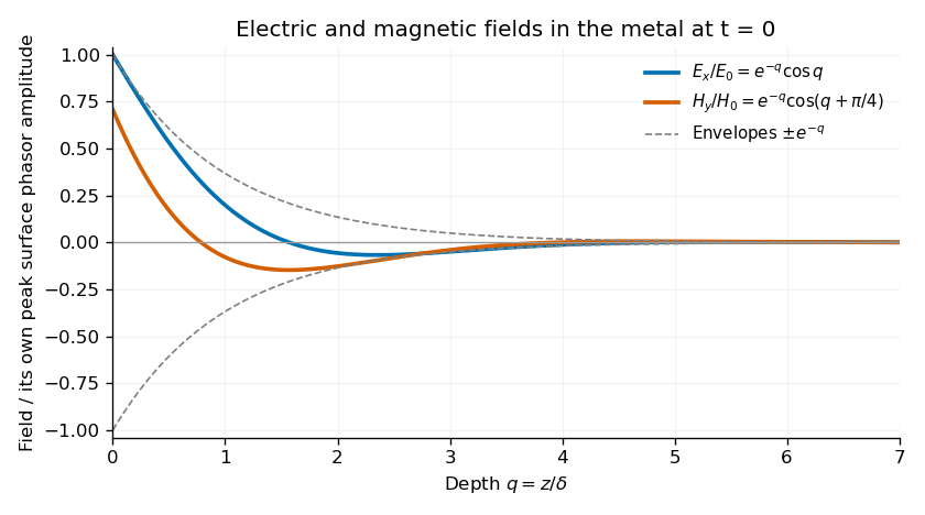
Original normalized electric and magnetic field profiles inside a good conductor at one instant, showing their common decay envelope and quarter-of-a-right-angle phase difference
. Details. 
An individual travelling wave in the lossless exterior has no attenuation, real wave impedance and in-phase electric and magnetic fields. The exterior total field also includes the reflected wave and may show interference, so it need not share that simple phase relation everywhere. At the interface the tangential fields match; is the field just inside the metal, not necessarily the incident amplitude. A good conductor reflects strongly and its wave impedance is much smaller than the vacuum impedance.
Average inward energy flux. For peak phasors, the Poynting vector averaged over a cycle is . The fields giveConsequently the constant in the question isThe flux is in the direction and has units .
Local energy conservation. The Poynting flux and local heating in a skin layer satisfyThe decrease becomes Joule heating in each layer. The Poynting theorem includes this transfer from field energy to the metal; averaged electromagnetic energy storage has zero time derivative in the periodic state, so no energy is lost from the complete balance.
Distributed line parameters. The geometry is the wide parallel-plate transmission line described in the question, with absolute permittivity . A length has charge and field , givingThe opposed plate currents have sheet density and confine the leading magnetic field between the plates. The magnetic energy per unit length is , soHere and are per unit length, in and , not lumped component values. Internal conductor fields and edge corrections are neglected.
Voltage and current evolution. The current entering a short length minus that leaving it is the rate of increase of its plate charge:The voltage drop across that length is its inductive drop, . Dividing by gives the lossless Telegrapher's equations,
Propagation speed. Differentiate these equations once more and eliminate the other variable:The wave equation speed is
Travelling-wave impedance. For a forward wave , take . Substitution into gives , hence the characteristic impedanceThe backward-wave current has the opposite sign relative to its voltage; the fixed ratio above applies to one travelling direction.
Matching the antenna. The voltage reflection coefficient is . No reflection requires . With , , and ,The resulting is consistent with the wide-plate approximation.
Both transverse forces. The matched transverse electromagnetic mode has electric attraction and magnetic repulsion. For time-averaged power ,The force on one plate excludes its own field. Thus the average electric attraction and magnetic repulsion per unit length are respectivelyThe electric and magnetic pressure cancellation in a matched TEM line follows directly from :The equality also holds instantaneously for a single travelling wave. Quoting either alone would omit the opposing contribution. This is the ideal electromagnetic force in the stated lossless uniform-dielectric model; a standing wave would not generally have the same cancellation.
Inertia and principal directions. About the centre of mass, the inertia tensor isIt relates angular momentum and angular velocity by and gives rotational kinetic energy . The principal axes are orthogonal eigenvector directions of this real symmetric tensor; in that basis it is diagonal, with entries the principal moments of inertia .
Derivatives in a rotating frame. Write in a body-fixed orthonormal basis. Each basis vector rotates according to . Differentiating the components and basis separately proves the rotating-frame derivative formula,The body derivative differentiates the scalar components in that basis. A fixed pivot can replace the centre of mass when the corresponding angular-momentum balance is valid.
Euler equations. The inertial angular-momentum equation is . Since the principal moments are constant in the body frame, substitute :These are Euler's equations in the principal body frame.
Linear perturbation of free rotation. After the impulse, . Let to leading order and be small. The third Euler equation changes only at quadratic order, so the linear transverse equations areFor and , eliminate fromThis givesIts units are inverse square seconds. Positive gives a growing real exponential; negative gives bounded oscillatory perturbations.
For three distinct positive principal moments of inertia, the denominator of is positive. If is the largest moment, the two numerator factors have opposite signs, so . If it is the smallest, they again have opposite signs. If is intermediate, the two factors have the same sign, so . Thus the intermediate axis theorem givesFor the stable cases the body-frame wobble frequency isThe perturbation does not decay in the torque-free conservative model. For the intermediate moment, a generic small impulse excites the growing branch and eventually leaves the linear regime.
Put , with . ThenRotation about the symmetry axis is stable whether that axial moment is larger or smaller than the transverse moment. In fact and are exactly constant for a torque-free axisymmetric body: the transverse components rotate into one another at the stated body-frame frequency. Stability here means bounded wobble, not relaxation back to perfect axial rotation.
Both the magnitude of angular momentum and rotational kinetic energy are conserved after the impulse. At fixed , eliminate to writeThe fixed-angular-momentum energy test for principal-axis rotation makes the stability geometric. The largest moment gives a constrained energy minimum, the smallest a maximum, and the intermediate moment a saddle. Conservation of energy keeps a nearby motion near either isolated extremum, but a saddle permits departure in one direction while compensating in another. Thus both extremes are stable without dissipation; it would be incorrect to demand an energy minimum alone in this conservative problem.
The differential gravitational acceleration responsible for a tidal force is the difference between accelerations at separated points of a body. Relative to a freely falling reference point , a small offset experiencesThe tidal tensor has units ; the vector called in the source is the resulting differential acceleration, in . An actual differential force is this vector multiplied by the test mass. Measurable effects include relative motion of separated freely falling masses, radial stretching, transverse squeezing, deformation and, when self-gravity or strength is insufficient, disruption. A spatially uniform acceleration alone produces no tidal deformation.
For a point mass, . Along the outward radial direction, andThus a small radial displacement has differential accelerationThe farther point falls inward less strongly, so its acceleration relative to the reference point points outward. The formula is first order in .
Take a transverse offset . Its distance from the source changes only at second order, but the direction of the gravitational force changes at first order:in its first-order vector expansion. Subtracting the reference acceleration givesIt compresses the transverse separation. Together with the radial result, this is point-mass tidal stretching and squeezing, with tensor eigenvalues .
The extra radial term. A circular Kepler orbit has . In the frame rotating with the synchronously spinning body, centrifugal acceleration increases by across a radial offset . This adds the outward differential accelerationEquivalently, in the inertial frame the farther corotating point needs an extra inward centripetal acceleration , which gravity alone does not supply. The total radial stretching relevant to the static corotating body is therefore . This is the corotating point-mass tidal field. The source's “force” expression is per unit mass.
Self-gravitational survival. Denote the asteroid radius by , distinct from the orbital radius . Its mass is and its surface self-gravitational acceleration is . Compare this restoring acceleration with radial tidal stretching :The corotating tidal-disruption estimate for a uniform sphere isThis is the requested spherical local force-balance estimate, not an exact fluid Roche figure. It neglects deformation and material cohesion.
Why the asteroid radius cancels. At fixed density, self-gravitational surface acceleration scales as . The linear tidal acceleration also scales as . Their ratio is therefore independent of , provided so that the tidal expansion is valid. Density, rather than asteroid size, controls this estimate.
The terrestrial value. Convert to and use :This is distance from Earth's centre, not height above its surface.
Compression and stretch viewed on rotated faces. To isolate shear, take equal small principal strains , . A square with sides at to these directions becomes a rhombus: adjacent side lengths are unchanged to first order, but their right angle changes by . In axes rotated through , the same strain tensor has zero diagonal entries and off-diagonal entries of magnitude .
The pure shear from opposite principal strains therefore has engineering shear strain , not . Equal opposite principal stresses give purely tangential traction of magnitude on those rotated faces. HenceIf the compression and stretch are not equal and opposite, an additional dilatational strain remains; their deviatoric part still supplies shear.
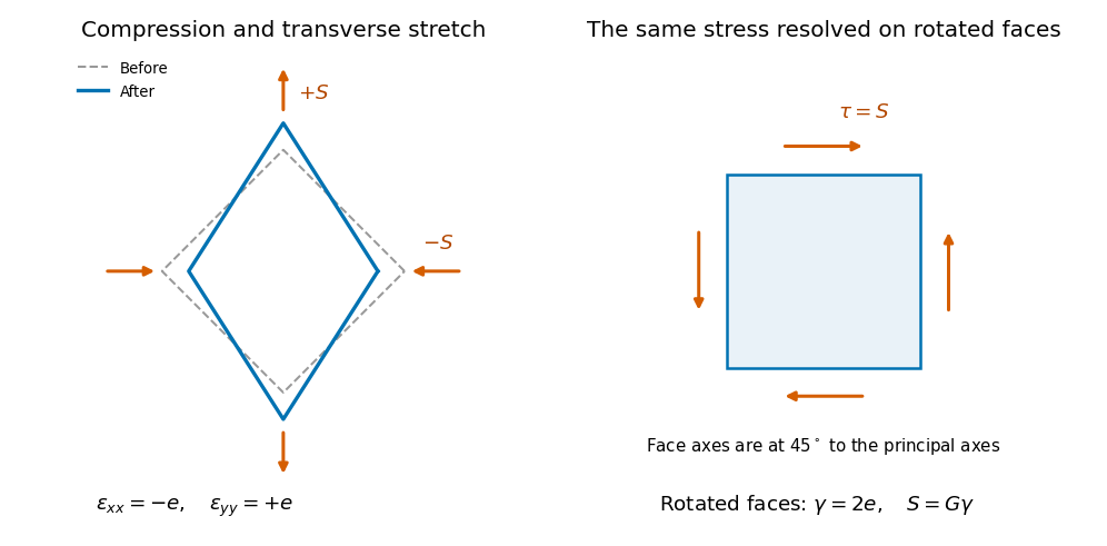
Original comparison of compression and transverse extension with the same stress resolved as shear on faces rotated through 45 degrees; deformation is exaggerated
. Details. 
The shaft's torsional stiffness. At radius , an end twist over length gives tangential displacement and shear angle . The local shear stress is . An annular area contributes torque , soThus torsion of a solid circular shaft givesHere is the polar second moment of area, in , not a mass moment of inertia. This is the transmitted torque magnitude; the shaft's restoring couple opposes the twist. The formula assumes small elastic shear and a circular uniform section.
Power is transmitted at rate , soFor , and , the polar second moment of area is . HenceThe density does not enter this static torsional deformation.
The torque rises linearly with elastic twist, so the stored elastic energy is the work integralUsing the transmitted torque and end twist,This is energy associated with deformation, distinct from the much larger kinetic energy of the whole spinning shaft.
For the uniform solid cylinder, the axial moment of inertia isThe rotational kinetic energy at isThis includes the shaft's bulk steady rotation; the small twist does not appreciably alter its mass moment at this order.
The torque difference. Let now be the local angular displacement, and take and the section constant. The local twist per unit length is , so the transmitted torque is . Across a short slice,Thusto first order in slice length.
The slice's angular acceleration. The slice's axial moment of inertia is . Its net torque is the difference of the end torques, soCanceling the common geometry gives the torsional waves in a solid circular rod,For the given steel, . The radius cancels because both torsional stiffness and slice inertia contain the same . This ideal one-dimensional wave model neglects dissipation and additional elastic modes.
Meaning and microscopic origin. For a Newtonian fluid, the dynamic viscosity measures tangential momentum transfer between fluid layers moving at different speeds. For the Newtonian shear considered here, , with units for . Molecular motion and collisions transport momentum across layers in a gas; intermolecular interactions contribute strongly in liquids. The resulting viscous forces oppose relative shear motion and convert organized kinetic energy to heat. The constitutive law is Newtonian and isotropic; incompressibility alone does not establish it.
Vertical force balance. Choose downward, as in the original diagram, and outward normal to the plate. In a uniform steady film, has zero advective acceleration and no along-plate pressure gradient. On a slice of thickness , the net shear force per unit face area is , while its weight per unit area is . ThereforeHere denotes the downward traction on a face with positive normal. The opposite face has the opposite traction orientation, accounting for the sign in the force difference.
Boundary conditions. At the fixed solid wall, the no-slip boundary condition is , with no normal penetration. At the free surface , neglect air shear, so and hence . The flat free surface has normal pressure , neglecting surface-curvature effects. These are a velocity condition at the wall and a stress condition at the free surface, not zero velocity at both boundaries.
The parabolic speed profile. Integrating from the shear-free surface gives . Thusand the wall condition yieldsIt is zero at the wall and largest at the free surface, where its gradient vanishes. The wall shear supports the downslope weight of the film per unit plate area.
Volume flux per unit width. Integrate through the depth:This is volume flow per unit length in , with units .
Inclining the plate. Keep normal outward from the plate and use downslope. The gravitational components are downslope and normal to the plate. For a uniform film of normal thickness , the steady slice equations areThe free-surface pressure condition givesUniform makes . The same no-slip and zero-surface-shear conditions then give the uniform gravity-driven Newtonian film,The component normal to the plate changes the hydrostatic pressure, while the tangential component drives the flow. The thickness is measured normal to the tilted plate.
The inclined-film volume flux. Integrating the new profile givesIt recovers the vertical result at and vanishes on a horizontal plate at fixed uniform depth. A varying depth, imposed pressure gradient or significant air shear would require additional terms; the solution here uses the uniform film specified by the simple draining-plate model.
Articles by others on the same topic
There are currently no matching articles.