Past exam of the physics of atmospheres and oceans course of the University of Oxford / 2022 / 6

Use a shallow, homogeneous active upper layer of mean thickness $h_0$ and mass density ${\rho }_1$, over a much deeper, effectively stationary layer with mass density ${\rho }_2>{\rho }_1$. The Boussinesq approximation keeps the small density contrast only in buoyancy, giving reduced gravity $g^{\prime }=g({\rho }_2-{\rho }_1)/{\rho }_0$. The hydrostatic approximation and shallow-water approximation make horizontal velocity nearly depth independent and turn the interface slope into the horizontal force $-g^{\prime }\nabla h$.

Linearize about rest and uniform $h_0$, with $|h-h_0|\ll h_0$, neglecting products of perturbations and convective acceleration. The f-plane approximation sets the Coriolis parameter to constant $f_0$. Neglect wind forcing, viscosity, entrainment and bottom drag. The two horizontal momentum equations then balance local acceleration, the Coriolis force and the pressure gradient. The signs $-f_{0}v$ and $+f_{0}u$ follow from eastward and northward coordinates.

The thickness equation is the linearized conservation of mass law: horizontal divergence decreases $h$, while horizontal convergence increases it. Here $h$ is active-layer thickness, not total ocean depth, and $g^{\prime }$ rather than $g$ gives the restoring force because the motion principally displaces the thermocline.

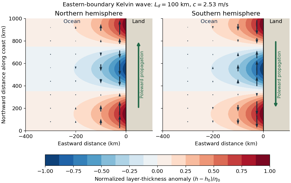
Put $\eta =h-h_0$ and $c=\sqrt{g^{\prime }{h}_0}$. With $u=0$ and complex dependence $e^{i({\omega }_{K}t-{\ell }_{K}y)}$, the northward momentum equation and continuity equation giveThus ${\omega }_K^2=c^2{\ell }_K^2$. Write the signed phase velocity as $c_y={\omega }_K/{\ell }_K=\pm c$, so $v=(c_y/h_0)\eta$. The eastward momentum equation is the transverse geostrophic balance $g^{\prime }{\eta }_x=f_{0}v$. HenceThe decaying sign is selected by which side of $x_b$ contains the ocean. For an eastern boundary the ocean occupies $x<x_b$, so decay offshore requires $f_0/c_y>0$. Consequently the Kelvin wave moves northwards in the northern hemisphere and southwards in the southern hemisphere, with the coast respectively on its right and left. The positive offshore decay length isThe sign of $f_0$ reverses the propagation direction and the sign of $v$ relative to $\eta$, but not the speed or offshore decay length. The real physical fields are the real parts of the complex solution. At the equator itself this local f-plane coastal solution loses its finite trapping scale.

Use Earth's rotation rate $\Omega =7.292\times 10^{-5}{\mathrm{s}}^{-1}$ and the Coriolis parameter $f=2\Omega \sin \varphi$. At $|\varphi |=10^{\circ }$,The Kelvin waves propagate polewards along the eastern boundary: northwards at $10^{\circ }$ N and southwards at $10^{\circ }$ S. The positive Rossby deformation radius uses $|f|$; the source's expression $c/f$ must be interpreted as a magnitude in the southern hemisphere.

The east-west e-folding distance is approximately $100$ km, orof longitude. With the coast at $x=0$ and ocean at $x<0$, a northern-hemisphere snapshot can be writtenAt a positive thickness crest, the thermocline is depressed and the alongshore velocity points polewards; a negative thickness trough reverses that velocity. In the southern hemisphere replace $c$ by $-c$ in the propagation and in $v/\eta$. The envelopes of both thickness and alongshore velocity decay offshore, and the cross-shore velocity vanishes.

Coastal Kelvin-wave radiation of long Rossby waves requires a common phase convention to match the two waves. The supplied Rossby wave formula conventionally multiplies $e^{i(k_{R}x+{\ell }_{R}y-{\omega }_{R}t)}$, while the coastal expression uses $e^{i({\omega }_{K}t-{\ell }_{K}y)}$. Since physical fields are real, matching may use the complex-conjugate representative; in either convention the boundary forcing fixes the absolute frequency and alongshore wavenumber. Thus $|{\omega }_R|=|{\omega }_K|$ and $|{\ell }_R|=|{\ell }_K|$.

For $k_R^2+{\ell }_R^2\ll L_d^{-2}$, the shallow-water Rossby-wave dispersion relation reduces toChoosing $k_R>0$ recovers the printed magnitude relation. Both the zonal phase velocity and zonal group velocity are approximately $-\beta L_d^2$, so the long Rossby waves carry the coastal signal westwards into the basin.

The coastal condition $|{\ell }_K|L_d\ll 1$ alone does not guarantee a long zonal wavelength. Since $|{\omega }_K|=c|{\ell }_K|$, matching requires $|k_R|=c|{\ell }_K|/(\beta L_d^2)$ and hence the stronger consistency conditionFor example, at $10^{\circ }$ a coastal wavenumber with $|{\ell }_K|L_d=0.05$ gives $|k_R|L_d\simeq 0.56$, which is not asymptotically small even though the meridional wavelength is long. Thus the source's proposed excitation is possible at sufficiently low frequency; it is not an automatic consequence of its meridional long-wave assumption.

At $10^{\circ }$ N or S the beta plane parameter isTaking a representative Pacific basin width $W\simeq 1.5\times 10^7$ m givesA width of $1.4$–$1.7\times 10^7$ m gives roughly $2.0$–$2.4$ years. This is propagation near $10^{\circ }$ latitude, not an equatorial $f=0$ calculation. Slow Rossby wave adjustment supplies a basin-scale delay relevant to El Niño–Southern Oscillation: changing thermocline depth can affect later sea surface temperature and coupled wind forcing. Reflection and coupling may help produce interannual memory, but this travel-time estimate alone does not establish a climate oscillation or its period.