Source bundle pages 40–47. The cover establishes 2022 despite the attachment filename. Solutions use the source notation; approximation limits and normalization conventions are stated where they affect the result.
For the variable-latent-heat saturation curve of a pure saturated water atmosphere, the total pressure equals the saturation pressure. The exact Clausius-Clapeyron relation along the phase coexistence curve iswhere are the specific volumes of the vapor and condensed thermodynamic phase. Neglecting and using the ideal gas law, , givesThe triple point provides the integration constant. Below it, the prescribed latent heat is constant, soAbove it, write . Integrating givesThese are the requested implicit temperature profiles . Both branches meet at , and each is monotone before the limiting liquid-gas critical point. The lower branch describes equilibrium with ice, rather than a stable liquid surface. A stable liquid ocean surface belongs to the upper branch; the colder upper atmosphere may use the lower branch. Hydrostatic balance is needed to convert this relation into a height profile, but not to obtain .
Let . For the temperature-dependent latent heat,Keeping the latent heat of vaporization fixed changes only the upper branch toBoth curves fall from as , pass through at the triple point, and are convex. At the triple point there is a corner because the latent heat changes from to . Their right-hand slopes there agree. Above the triple point,The variable-latent heat curve lies above the fixed-latent heat curve: its downward slope has smaller magnitude at every . It reaches a horizontal tangent at , whereas the fixed-latent heat curve is still descending. Both limiting ordinates are finite; this model gives and . These are extrapolations of the stipulated model, not accurate water liquid-gas critical point data. Extending the variable branch beyond would give negative latent heat and is physically inadmissible.
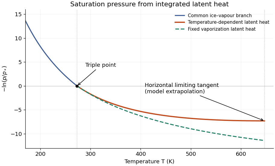
For constant gravitational acceleration, hydrostatic balance gives the atmospheric column mass , with negligible pressure at the top. For the same surface temperature , the variable latent heat gives a smaller integrated , and henceMultiplying by the same planetary surface area gives the same comparison for total mass. The models agree for a surface at or below the triple point, where they use the same sublimation branch. The comparison assumes the same surface temperature, rather than the same surface pressure.
No. Near the liquid-gas critical point, the mass densities of liquid and vapor approach each other, so the neglected condensed-phase specific volume becomes comparable with the vapor specific volume. The vapor also ceases to obey the dilute ideal gas law. Although the latent heat tends to zero, the specific-volume difference tends to zero too: the exact Clausius-Clapeyron relation contains their ratio. Setting only the numerator to zero therefore does not justify a vanishing physical saturation pressure slope. A realistic equation of state and coexistence data are required near the surface; the dilute colder upper atmosphere can still be described approximately by the earlier expression.
The pressure-linear grey opacity model interprets as a mass absorption coefficient. If it is instead a molecular absorption cross section, replace below by that cross section divided by molecular mass. Assume a plane-parallel atmosphere, hydrostatic balance, local thermodynamic equilibrium, and thermal absorption and emission without scattering of light. With height increasing upwards,Integrating upwards from the surface givesThusThe vertical optical depth is dimensionless. The atmosphere is optically thick when and optically thin when . A ray with zenith-angle cosine sees optical depth , so even a vertically thin layer can be opaque along a sufficiently grazing ray.
It is convenient to use the optical depth above a level,Thermal radiation escapes mainly from levels with of order unity: emission much deeper is attenuated, while the column far above contains little emitting material. Hence, in an optically thick atmosphere,For a particular viewing direction, instead gives . These are characteristic levels, not sharp emitting surfaces; the contribution function depends on the temperature exponent . If , the formal level lies below the surface and the surface itself contributes strongly. A useful estimate then clips at .
Write , , and . The integrated Planck function is by the Stefan–Boltzmann law, andThe formal radiative transfer equation solution for upward radiance at the top isThe first term is transmitted surface emission; the second is emission from the atmosphere. Integrating radiance over the upward hemisphere gives the outgoing radiant flux per unit area,Here is an exponential integral. For fixed and , surface transmission is negligible and the upper limit can be extended to infinity. Positivity permits interchanging the integrals; putting givesConsequently the exact hemispheric optically thick result isThis is a dimensional scale times a dimensionless definite integral depending only on . In the commonly used vertical-ray approximation, define . ThenA vertical-ray approximation therefore has the same scaling but omits the angular factor . Stating which quantity is used prevents a purely angular normalization discrepancy.
At fixed and , the outgoing radiant flux scales as . Increasing the optical depth shifts the effective emitting region to lower pressure and lower temperature. A surface temperature cannot be inferred from emission alone: specify the absorbed stellar radiant flux and impose radiative equilibrium, . If the no-atmosphere blackbody has , thenThe vertical-ray approximation omits from this prefactor. For fixed and sufficiently large optical depth, the surface is warmer than : this is the thermal greenhouse effect within the prescribed temperature profile. It does not by itself establish a self-consistent vertical heating or convection balance.
For , put . Repeated integration by parts gives . The hemispheric thick-limit results areThe second row assumes fixed surface temperature; the third assumes fixed absorbed radiant flux. In the vertical-ray approximation the first of these rows becomes , and the surface temperature factors are the inverse fourth roots.
Thus increasing makes the atmosphere colder at every fixed , decreases outgoing radiation at fixed , and requires a warmer surface at fixed absorbed radiant flux. The case is isothermal and gives exactly, including finite optical depth.
There is an essential approximation limit. The extension of the integral to infinity is valid for fixed as , and is not uniform for arbitrarily large at fixed . The vertical integrand peaks at , so one needs that peak well above the surface in optical depth, with a negligible tail beyond . For example, at the thick formula predicts for but approximately for . This artificial increase contradicts the exact monotonicity: in the finite-optical depth expression every atmospheric emission factor decreases with . At fixed finite , the exact limiting outgoing radiant flux is the transmitted surface term , rather than factorial divergence.
The dilute Köhler curve follows because the Kelvin equation multiplies the planar-solution saturation pressure by the curvature correction. Combining it with Raoult's law therefore givesFor a dilute chemical solution and a small curvature correction, and . A first-order Taylor expansion givesThus the simplified Köhler theory relation isThe curvature term raises the required ambient vapor pressure; the solute term lowers it. These laws combine multiplicatively before linearization, so the displayed simplified relation is an approximation, not an exact identity.
For , differentiating the simplified Köhler theory curve givesThe derivative is positive below and negative above it, so is the Köhler activation radius, the unique maximum. At that point , givingThe curve crosses at , reaches at , and approaches from above as . Its formal divergence to negative values as is outside the dilute-chemical solution approximation; a finite dry solute core and composition-dependent properties must replace that extrapolation.
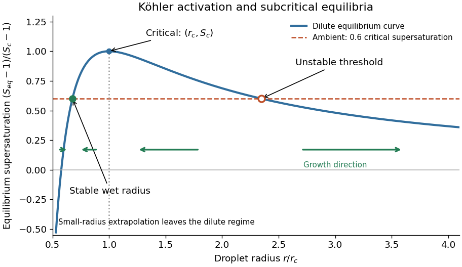
Köhler equilibrium curve and growth directions at subcritical supersaturation
. Details. Let be the ambient saturation ratio. There are two equilibrium radii: . Condensation occurs if ; evaporation occurs if . Therefore droplets with grow towards , while those with shrink towards . The smaller equilibrium is stable.
Above , droplets with still undergo evaporation and ultimately approach . Droplets with grow, and the larger equilibrium is unstable. Merely exceeding is therefore not sufficient for continued growth at subcritical ambient atmospheric supersaturation. For example, if , the two intersections have approximately and ; a droplet of radius undergoes evaporation. If instead , there is no equilibrium barrier in this approximation and droplets activate into growing cloud droplets.
Köhler theory explains activation of cloud condensation nuclei, rather than rapid production of atmospheric precipitation. Diffusion-controlled droplet growth is limited by diffusion of water vapor and removal of released latent heat; approximately is proportional to the ambient atmospheric supersaturation. It slows in radius and tends to narrow a droplet size distribution. The available water vapor, changing temperature and shared depletion of atmospheric supersaturation also invalidate unlimited growth at prescribed . Formation of rain-sized drops normally requires collision-coalescence, while colder clouds can additionally use cloud ice nucleation versus ice growth.
At the Köhler activation radius, the two coefficients satisfyConverting the atmospheric supersaturation to a fraction gives , not . Henceand the supplied curvature coefficient gives the temperatureThe coefficient and the stated radius consistently use a radius convention; replacing radius by diameter without changing the coefficient would introduce a factor-of-two error.
A Michelson interferometer uses a beam splitter to divide collimated input light between a fixed mirror and a moving mirror. Returning beams recombine at the beam splitter; one output reaches a photodetector. A compensator plate can equalize the glass traversed in the two arms. Moving one mirror by changes the optical path difference by .
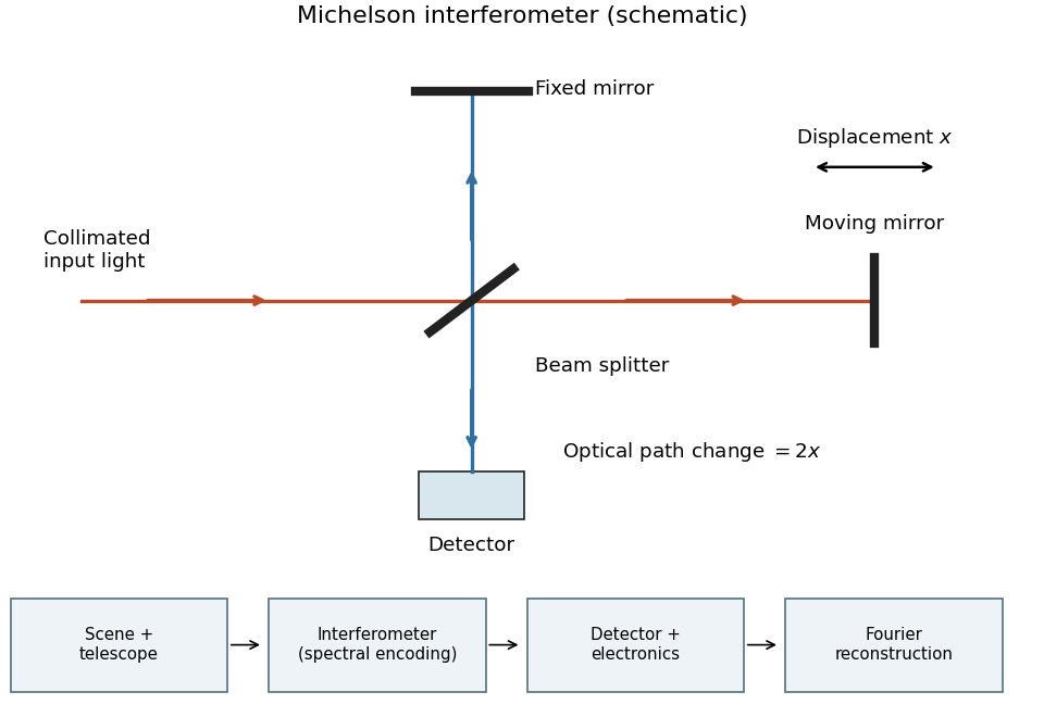
Michelson interferometer and the corresponding measurement chain
. Details. The usual nominal Fourier transform spectroscopy specification is , where is the maximum optical path difference measured from equal arms. It givesThis is a nominal spectral resolution element convention.[ref]
FTIR Moving Mirror Travel Distance Calculation by Thermo Fisher Scientific. optical path difference equals reciprocal resolution; mirror travel is half the optical path difference
A symmetric rectangular scan from to instead has a sinc instrumental line shape with first-zero offset . Quoting that first-zero criterion would give cm; interferogram apodization and other linewidth criteria change the numerical factor. An exact mathematical minimum requires such a criterion.In the measurement chain, the Michelson interferometer is the spectral analyzer or modulator, between the collection optics and the photodetector. It encodes the incoming radiation spectrum into an interferogram; detector electronics digitize that signal and a Fourier transform reconstructs the radiation spectrum. It does not itself turn radiant power into an electrical signal.
Let the two returning monochromatic fields at the chosen detector port beHere is wavenumber, rather than temporal frequency. An optical-cycle average uses and . In units absorbing the detector's field-to-power conversion,The choice of output port can reverse the cosine sign. For mutually incoherent components of the radiation spectrum, add powers rather than instantaneous fields, givingSubtracting the constant term leaves the Fourier cosine transform of the detected spectral weighting , including throughput and detector response.
The printed prefactor requires a normalization convention. In the derivation, is the amplitude of each returning field at the detector, not an entrance amplitude with input power . For a lossless balanced beam splitter and literal input power , conservation of energy instead gives , so the source formula identifies . Taking both and the printed formula literally would give at zero optical path difference, a concrete normalization contradiction.
Ignoring refraction, the line of sight is perpendicular to the radius at its tangent point. For a surface tangent, Pythagorean theorem gives the satellite-to-tangent distanceFor tangent altitude , replace by ; lower atmospheric scale heights change the estimate little. The required angular resolution isUsing the Rayleigh criterion for a circular telescope aperture, . The longest wavelength imposes the strongest condition, soThe corresponding requirement at is mm. This is a diffraction limit, without allowance for scan sampling, aberrations or instrumental field of view.
Use one spectral resolution element, , and assume comparable angular resolution horizontally and vertically, so the pixel solid angle is . The question specifies only the vertical angle; without an assumption about horizontal field of view the diameter is not unique. Interpret throughput as dimensionless transmission. With primary collecting area , the power in that element iswhen is in square metres. There is no extra factor of multiplying the supplied spectral radiance.
For an integration time s, the order-of-magnitude effective noise bandwidth is Hz. The root-mean-square noise-equivalent power is then W.[ref]
NEP – Noise Equivalent Power by Thorlabs. p. 1, NEP Definition; p. 2, equations (2)–(3): minimum power and averaging time
A signal-to-noise ratio of 10 requires W, and thereforeAn ideal rectangular average of a one-sided white noise spectral density has , giving cm instead. A circular field with diameter changes the diameter by another order-unity factor. These convention choices all require an aperture substantially larger than the mm diffraction estimate, so signal collection is the stronger constraint. The estimate treats the quoted NEP as applicable to the reconstructed channel; a detailed Fourier transform spectroscopy design would also specify scan weighting, background and how interferogram noise propagates into that channel.The constants are effective reservoir capacities: stored carbon dioxide mass anomaly per unit effective concentration anomaly, in GtCO per ppmv. Only is a literal atmospheric mole fraction; are scaled reservoir variables chosen to share its equilibrium value. The exchange coefficients are conductances, in GtCO per ppmv per year: is transfer from the atmosphere to the fast reservoir and transfer from that reservoir to the deep ocean. They are not by themselves inverse times; division by a reservoir capacity gives an inverse-time rate.
Hydrostatic balance estimates total atmospheric mass as . One ppmv of a dilute ideal gas is a mole fraction , so, with dry-air molar mass g/mol and carbon dioxide molar mass g/mol,The final factor converts kilograms to gigatonnes. This is carbon dioxide mass, not the smaller carbon mass.
For the linear three-reservoir carbon model, with concentrations as a column vector, the linear ordinary differential equation isA homogeneous normal mode has , where . For negative real eigenvalues the e-folding relaxation time is . The row sums vanish, so has andEqual effective concentrations generate no exchange. Summing the reservoir budgets givesThus injected carbon dioxide is conserved after emissions cease: the model redistributes it but contains no permanent removal. The zero normal mode records this conserved excess mass, rather than a long but finite decay.
To check the other normal modes are damped, set and . ThenThe similarity transformation is a symmetric negative-semidefinite matrix with a one-dimensional kernel, so the remaining two eigenvalues are strictly negative.
Define the two concentration differences and . For zero emissions and , their ordinary differential equation isWriting the positive decay rates as , their characteristic equation isConsequentlyFor , the first normal mode rapidly equalizes the fast reservoirs, giving . The slower evolution treats them as a combined capacity exchanging with , giving . ThereforeThe timescale ratio is in the joint limit. Since the conserved normal mode has , the hierarchy is .
Here , , , and , in the stated reservoir units. The exact characteristic coefficients are and , givingThe leading separation estimates give yr and yr if finite is retained, or yr if is also sent to infinity. Thus ; a ratio of ten warrants using the exact values for the requested sketch.
Assume initially zero anomalies in all reservoirs. The atmospheric impulse response, obtained by decomposing into the three normal modes, iswith , , and , in ppmv/GtCO. The checks and fix the instantaneous injection response and its initial decay.
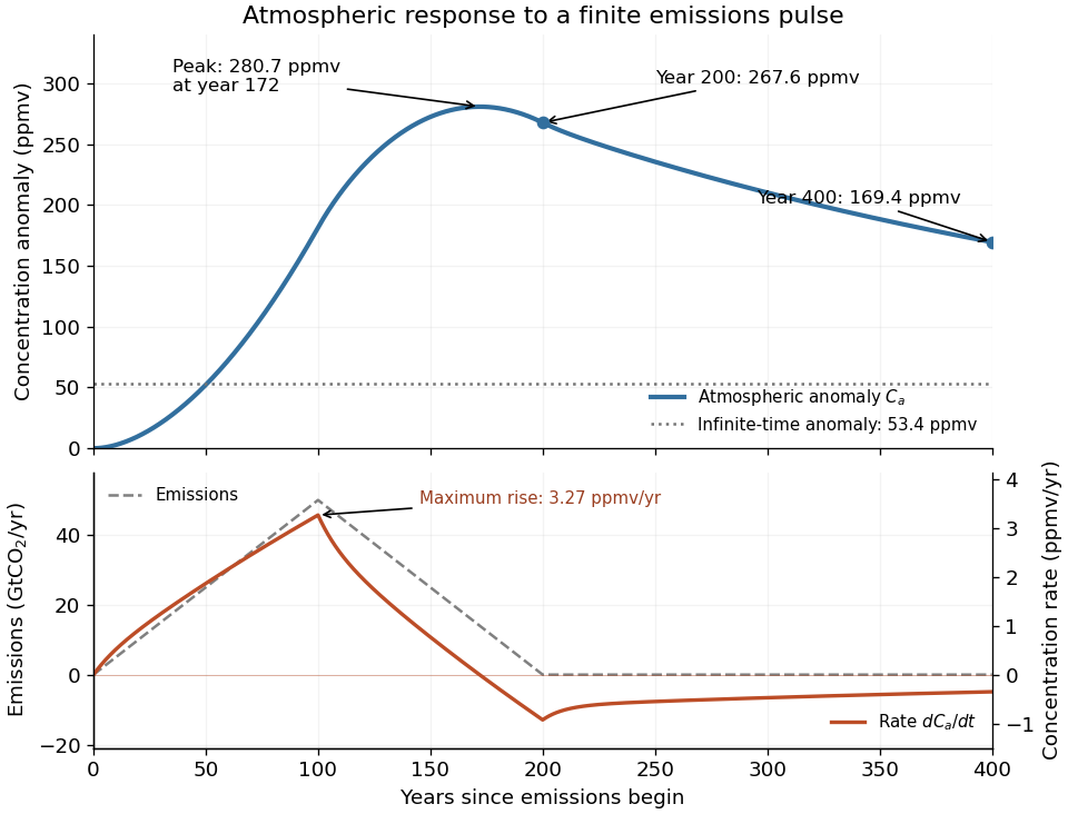
The concentration is the convolution . To evaluate it transparently, define for , andsetting every when . Expressing the triangular emission history as givesHere times are in years and has the corresponding emission-ramp units. Differentiating or evaluating the convolution givesThe maximum concentration occurs earlier than the end of emissions, at approximately year , with ppmv. Initially there is a short adjustment over ; the curve then rises, turns over as emissions fall, and continues declining after year 200 as the deep ocean takes up carbon dioxide.
The total emitted mass is the area of the emission triangle, GtCO. All reservoirs eventually share one concentration, so conservation of mass gives
Use a shallow, homogeneous active upper layer of mean thickness and mass density , over a much deeper, effectively stationary layer with mass density . The Boussinesq approximation keeps the small density contrast only in buoyancy, giving reduced gravity . The hydrostatic approximation and shallow-water approximation make horizontal velocity nearly depth independent and turn the interface slope into the horizontal force .
Linearize about rest and uniform , with , neglecting products of perturbations and convective acceleration. The f-plane approximation sets the Coriolis parameter to constant . Neglect wind forcing, viscosity, entrainment and bottom drag. The two horizontal momentum equations then balance local acceleration, the Coriolis force and the pressure gradient. The signs and follow from eastward and northward coordinates.
The thickness equation is the linearized conservation of mass law: horizontal divergence decreases , while horizontal convergence increases it. Here is active-layer thickness, not total ocean depth, and rather than gives the restoring force because the motion principally displaces the thermocline.
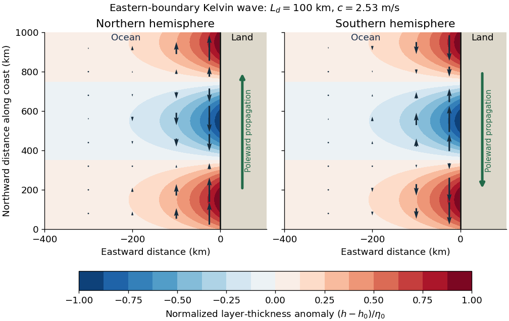
Put and . With and complex dependence , the northward momentum equation and continuity equation giveThus . Write the signed phase velocity as , so . The eastward momentum equation is the transverse geostrophic balance . HenceThe decaying sign is selected by which side of contains the ocean. For an eastern boundary the ocean occupies , so decay offshore requires . Consequently the Kelvin wave moves northwards in the northern hemisphere and southwards in the southern hemisphere, with the coast respectively on its right and left. The positive offshore decay length isThe sign of reverses the propagation direction and the sign of relative to , but not the speed or offshore decay length. The real physical fields are the real parts of the complex solution. At the equator itself this local f-plane coastal solution loses its finite trapping scale.
Use Earth's rotation rate and the Coriolis parameter . At ,The Kelvin waves propagate polewards along the eastern boundary: northwards at N and southwards at S. The positive Rossby deformation radius uses ; the source's expression must be interpreted as a magnitude in the southern hemisphere.
The east-west e-folding distance is approximately km, orof longitude. With the coast at and ocean at , a northern-hemisphere snapshot can be writtenAt a positive thickness crest, the thermocline is depressed and the alongshore velocity points polewards; a negative thickness trough reverses that velocity. In the southern hemisphere replace by in the propagation and in . The envelopes of both thickness and alongshore velocity decay offshore, and the cross-shore velocity vanishes.


Coastal Kelvin-wave radiation of long Rossby waves requires a common phase convention to match the two waves. The supplied Rossby wave formula conventionally multiplies , while the coastal expression uses . Since physical fields are real, matching may use the complex-conjugate representative; in either convention the boundary forcing fixes the absolute frequency and alongshore wavenumber. Thus and .
For , the shallow-water Rossby-wave dispersion relation reduces toChoosing recovers the printed magnitude relation. Both the zonal phase velocity and zonal group velocity are approximately , so the long Rossby waves carry the coastal signal westwards into the basin.
The coastal condition alone does not guarantee a long zonal wavelength. Since , matching requires and hence the stronger consistency conditionFor example, at a coastal wavenumber with gives , which is not asymptotically small even though the meridional wavelength is long. Thus the source's proposed excitation is possible at sufficiently low frequency; it is not an automatic consequence of its meridional long-wave assumption.
At N or S the beta plane parameter isTaking a representative Pacific basin width m givesA width of – m gives roughly – years. This is propagation near latitude, not an equatorial calculation. Slow Rossby wave adjustment supplies a basin-scale delay relevant to El Niño–Southern Oscillation: changing thermocline depth can affect later sea surface temperature and coupled wind forcing. Reflection and coupling may help produce interannual memory, but this travel-time estimate alone does not establish a climate oscillation or its period.
Articles by others on the same topic
There are currently no matching articles.