The hypocentre is the point where rupture begins. The epicentre is its projection onto the Earth's surface. An earthquake centroid is an effective spatial average of moment release over the rupture, with a corresponding mean release time. Initiation and average release need not occur at the same place or time, especially for an extended, asymmetric rupture.
Identify the event and pick calibrated P wave and, where available, S wave arrivals at stations of known position. Associate each pick with a seismic phase and uncertainty. An earthquake location by arrival times fitsfor the three hypocentre coordinates and earthquake origin time, using travel times from a specified velocity model. A grid search can initialize iterative weighted least squares or a probabilistic inversion. Station coverage must constrain depth as well as horizontal position; merely having four observations does not ensure a well-conditioned solution.
Errors include uncertain or misidentified onsets, clock and station-coordinate errors, wrong velocities or neglected three-dimensional structure, poor azimuthal coverage, inadequate station distances and depth–origin-time tradeoffs. Examine residual patterns and resolution, not only the minimum residual. A small formal covariance within a wrong velocity model can accompany a systematically biased hypocentre.
For a double-couple seismic source, measure P-wave first-motion polarity signs and use source-to-station takeoff angles from the location and velocity model to plot them on a focal sphere. Fit the alternating radiation-sign quadrants, optionally adding amplitude ratios and waveform information. The two nodal planes determine a focal mechanism, conventionally expressed by fault strike, fault dip and fault rake.
A more general waveform inversion fits a seismic moment tensor to several components and stations. Its double-couple part supplies candidate slip and normal vectors, but a general moment tensor should not be forced to be double-couple without justification. Polarity calibration, near-nodal observations, path effects and takeoff-angle errors limit the result.
Point-source radiation alone interchanges the fault plane and auxiliary plane without changing the double couple. Resolve this fault-plane ambiguity using mapped rupture, aftershock geometry, geodesy or finite-rupture directivity. A dense set of polarity picks does not by itself remove that fundamental ambiguity.
Linearized arrivals contain . When the stations have similar depth sensitivities, a depth change shifts nearly all predicted times together and an origin-time change compensates it. Distant stations can also have very weak depth sensitivity. Improve the range of takeoff angles and station distances, especially with nearby or borehole stations, and include S–P or depth-phase differences such as pP–P that cancel origin time while retaining depth information. Accurate phase identification and the velocity model remain necessary.
Nearby events observed at the same station share most of their propagation path, so common model and station errors cancel in differential arrival times. Waveform cross-correlation can also determine their relative timing more precisely than separate onset picks. Double-difference earthquake relocation fitsalong with the difference in origin times. The relative cluster geometry can be precise while the entire cluster remains displaced. Absolute anchoring still needs a well-calibrated velocity model or a source of known position.[ref]
A Double-difference Earthquake Location Algorithm: Method and Application to the Northern Hayward Fault, California by F. Waldhauser and W. Ellsworth. 2000, method and common-path rationale
Let the seismic moment tensor of a double-couple seismic source be for perpendicular unit slip and normal vectors. Its T axis is , with eigenvalue , and its P axis is , with eigenvalue . They bisect the fault-plane and auxiliary-plane quadrants.
These earthquake pressure and tension axes describe the source deformation. They are not generally the principal axes of the ambient stress tensor. Friction, inherited fault orientation and local stress changes can rotate their relationship to that tensor; a stress inversion requires further assumptions and multiple mechanisms.
A dense array does not correct an incorrect velocity model. The faster southwest block permits shorter travel times than an assumed uniform medium, with refraction favouring paths through fast rock. First arrivals may include refracted or seismic head wave paths rather than the assumed direct straight paths. Fitting those arrivals with one constant speed can make an earthquake on the fault appear closer to southwest stations and farther from northeast stations.
The sign follows even from a two-station linearization. Put southwest and northeast stations at , and the true event at with depth . In a constant-speed model,A negative observed differential residual therefore produces , an apparent southwest displacement. A common origin-time adjustment cannot remove this directional residual. The stated kilometre-scale offset is a model bias, not proof that the fault dips towards the apparent epicentres. Its exact magnitude cannot be predicted without the actual velocities and station geometry; the question supplies that magnitude as an observation.
The relevant contrast is independently documented at Parkfield: higher velocities lie southwest of the fault, with lower velocities northeast.[ref]
Scientific Advances at Parkfield by United States Geological Survey. Velocity-structure discussion, higher speeds southwest and lower speeds northeast
Account for the lateral structure and correct phases, then relocate and test whether the bias remains.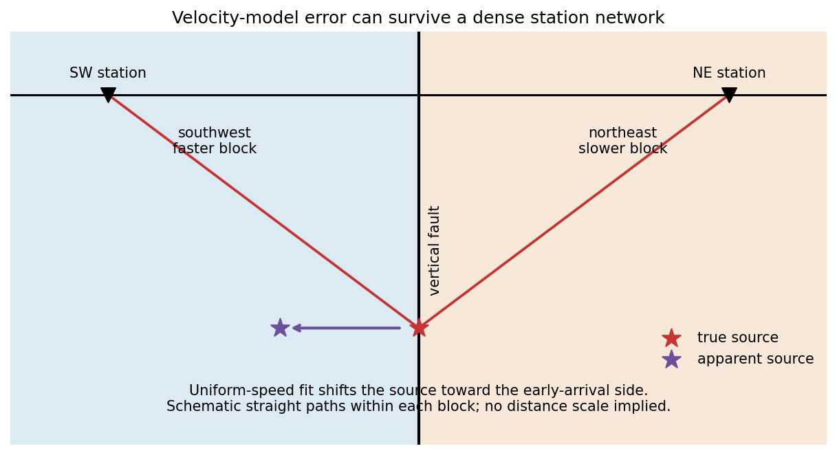

Articles by others on the same topic
There are currently no matching articles.