The hypocentre is the point where rupture begins. The epicentre is its projection onto the Earth's surface. An earthquake centroid is an effective spatial average of moment release over the rupture, with a corresponding mean release time. Initiation and average release need not occur at the same place or time, especially for an extended, asymmetric rupture.
Identify the event and pick calibrated P wave and, where available, S wave arrivals at stations of known position. Associate each pick with a seismic phase and uncertainty. An earthquake location by arrival times fitsfor the three hypocentre coordinates and earthquake origin time, using travel times from a specified velocity model. A grid search can initialize iterative weighted least squares or a probabilistic inversion. Station coverage must constrain depth as well as horizontal position; merely having four observations does not ensure a well-conditioned solution.
Errors include uncertain or misidentified onsets, clock and station-coordinate errors, wrong velocities or neglected three-dimensional structure, poor azimuthal coverage, inadequate station distances and depth–origin-time tradeoffs. Examine residual patterns and resolution, not only the minimum residual. A small formal covariance within a wrong velocity model can accompany a systematically biased hypocentre.
For a double-couple seismic source, measure P-wave first-motion polarity signs and use source-to-station takeoff angles from the location and velocity model to plot them on a focal sphere. Fit the alternating radiation-sign quadrants, optionally adding amplitude ratios and waveform information. The two nodal planes determine a focal mechanism, conventionally expressed by fault strike, fault dip and fault rake.
A more general waveform inversion fits a seismic moment tensor to several components and stations. Its double-couple part supplies candidate slip and normal vectors, but a general moment tensor should not be forced to be double-couple without justification. Polarity calibration, near-nodal observations, path effects and takeoff-angle errors limit the result.
Point-source radiation alone interchanges the fault plane and auxiliary plane without changing the double couple. Resolve this fault-plane ambiguity using mapped rupture, aftershock geometry, geodesy or finite-rupture directivity. A dense set of polarity picks does not by itself remove that fundamental ambiguity.
Linearized arrivals contain . When the stations have similar depth sensitivities, a depth change shifts nearly all predicted times together and an origin-time change compensates it. Distant stations can also have very weak depth sensitivity. Improve the range of takeoff angles and station distances, especially with nearby or borehole stations, and include S–P or depth-phase differences such as pP–P that cancel origin time while retaining depth information. Accurate phase identification and the velocity model remain necessary.
Nearby events observed at the same station share most of their propagation path, so common model and station errors cancel in differential arrival times. Waveform cross-correlation can also determine their relative timing more precisely than separate onset picks. Double-difference earthquake relocation fitsalong with the difference in origin times. The relative cluster geometry can be precise while the entire cluster remains displaced. Absolute anchoring still needs a well-calibrated velocity model or a source of known position.[ref]
A Double-difference Earthquake Location Algorithm: Method and Application to the Northern Hayward Fault, California by F. Waldhauser and W. Ellsworth. 2000, method and common-path rationale
Let the seismic moment tensor of a double-couple seismic source be for perpendicular unit slip and normal vectors. Its T axis is , with eigenvalue , and its P axis is , with eigenvalue . They bisect the fault-plane and auxiliary-plane quadrants.
These earthquake pressure and tension axes describe the source deformation. They are not generally the principal axes of the ambient stress tensor. Friction, inherited fault orientation and local stress changes can rotate their relationship to that tensor; a stress inversion requires further assumptions and multiple mechanisms.
A dense array does not correct an incorrect velocity model. The faster southwest block permits shorter travel times than an assumed uniform medium, with refraction favouring paths through fast rock. First arrivals may include refracted or seismic head wave paths rather than the assumed direct straight paths. Fitting those arrivals with one constant speed can make an earthquake on the fault appear closer to southwest stations and farther from northeast stations.
The sign follows even from a two-station linearization. Put southwest and northeast stations at , and the true event at with depth . In a constant-speed model,A negative observed differential residual therefore produces , an apparent southwest displacement. A common origin-time adjustment cannot remove this directional residual. The stated kilometre-scale offset is a model bias, not proof that the fault dips towards the apparent epicentres. Its exact magnitude cannot be predicted without the actual velocities and station geometry; the question supplies that magnitude as an observation.
The relevant contrast is independently documented at Parkfield: higher velocities lie southwest of the fault, with lower velocities northeast.[ref]
Scientific Advances at Parkfield by United States Geological Survey. Velocity-structure discussion, higher speeds southwest and lower speeds northeast
Account for the lateral structure and correct phases, then relocate and test whether the bias remains.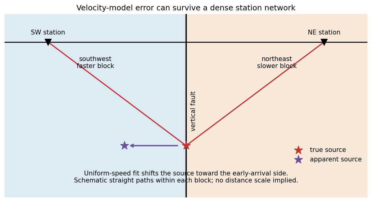
Ice accumulation adds a load that produces an immediate elastic response and slower viscous displacement of the mantle away from the loaded region. The depressed interior may be accompanied by a peripheral forebulge. A long-lived load approaches an approximately compensated state. Melting removes the load, giving rapid elastic recovery followed by mantle return flow and gradual uplift. The forebulge can subside while the formerly loaded centre rises.
Postglacial rebound can continue long after the ice disappears, because mantle relaxation is slow. Raised shorelines, changing relative sea level, vertical geodetic motion and gravity changes record glacial isostatic adjustment. Present motion depends on the whole loading and melting history, mantle rheology and lithospheric stiffness, not only the current absence of ice.
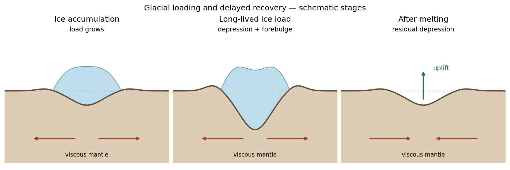


Subtract the background hydrostatic pressure. A relief amplitude produces a restoring pressure perturbation and horizontal gradient . Incompressibility makes the disturbance penetrate a depth of order its horizontal scale. For sinusoidal viscous rebound, with relaxation speed , the viscous force density is . Balancing givesThis is a small-amplitude viscous half-space estimate; numerical factors from the sinusoidal geometry are absent from a scaling argument.
Unsteady inertial force density scales as , whereas viscous force density scales as . Using the preceding timescale givesConvective inertia has ratio . Since , this is smaller by for small relief. Thus the displayed estimate controls the larger inertial contribution in this model.
Assume the original ice sheet had time to reach local isostatic compensation, melted rapidly relative to subsequent rebound, and left one exponentially relaxing depression mode. Neglect elastic layering and assign the whole present gravity deficit to that unrelaxed depression. Load balance givesThe supplied sheet-gravity approximation gives the residual amplitudeFrom ,For an order-of-magnitude single-mode estimate, choose the ice-sheet diameter as wavelength, . Taking , the more accurate specified relation then givesA circular load has a spectrum, not one uniquely specified wavelength. Choosing instead gives about ; another wavelength convention rescales the answer linearly. The robust inference is viscosity of order within this simple model. A realistic estimate would also model gradual melting, other gravity anomalies, density interfaces, lithospheric flexure and depth-dependent mantle viscosity.
Using the same diameter convention and viscosity estimate,Geometrical factors omitted in the scaling do not affect the conclusion: inertia is negligible. Convective inertia is smaller still by the small relief-to-wavelength ratio. Mantle creep is extremely slow despite the large length scale.
Elastic rebound. Tectonic motion loads a fault whose shallow portion is locked. Rock on either side deforms and stores elastic strain energy while slip is inhibited. When failure permits rapid slip, part of the stored energy becomes seismic radiation and part is dissipated in friction and damage. The adjacent rock partly relaxes, while a permanent displacement remains across the fault. Geodetic strain accumulation and coseismic offsets support this loading–release picture.[ref]
Reid's Elastic Rebound Theory by United States Geological Survey. Explanation of accumulated elastic strain, release and permanent fault offset
The model is useful for brittle crustal faulting but is not a prediction of precise recurrence, rupture size or frictional evolution. Aseismic creep can release deformation without a large sudden event. Viscoelastic flow, afterslip, fluid-pressure changes and interacting fault segments complicate a simple locked-fault cycle. Deep-focus earthquakes and non-shear source components require additional physics; not every earthquake source is adequately described by a shallow brittle double couple. Rebound also need not release all the pre-existing stress.
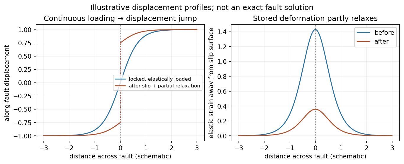
Original displacement-profile schematic of locked loading and permanent slip after relaxation
. Details. 
A thin negative-gradient velocity zone. In horizontal layering, use the seismic ray parameter , the conserved horizontal slowness. A ray turns when . Downward passage through decreasing speed makes smaller, so a surface ray cannot turn in the negative-gradient interior. Rays either turn above the zone or penetrate it and turn below where speed has recovered sufficiently. This produces missing turning depths and a seismic shadow range from a low-velocity zone in the ideal ray model.
Retain all branches usingThe travel-time slope is . Just below the critical value that permits passage beyond the upper speed maximum, the ray makes a finite extra excursion through the low-velocity region. Range can jump, and the deep branch can fold back before resuming its normal trend, giving multiple arrivals outside the shadow. A first-arrival curve alone hides some of these branches. Define the seismic intercept time byThe – representation displays the gap and fold; the – representation has separate shallow and deep branches and a branch jump at the critical ray parameter for the piecewise-linear cusp model. Do not join them by invented turning rays. Diffraction and finite-frequency energy soften a purely geometrical shadow.
The figures use an explicit illustrative profile, not measured Earth parameters: speed rises from 1 to 2 over depths 0 to 1, falls to 1.8 by depth 1.2, then rises with its original gradient. The asthenosphere beneath oceanic lithosphere is an important setting for a low-velocity zone. A major P-wave speed reduction also occurs at the boundary between the mantle and the outer core of the Earth; S waves do not propagate through the liquid outer core of the Earth.[ref]
Essentials of Geophysics: Seismology by R. D. van der Hilst. Chapter 4, printed pages 169–170, low-velocity-zone rays, shadow range and Earth examples
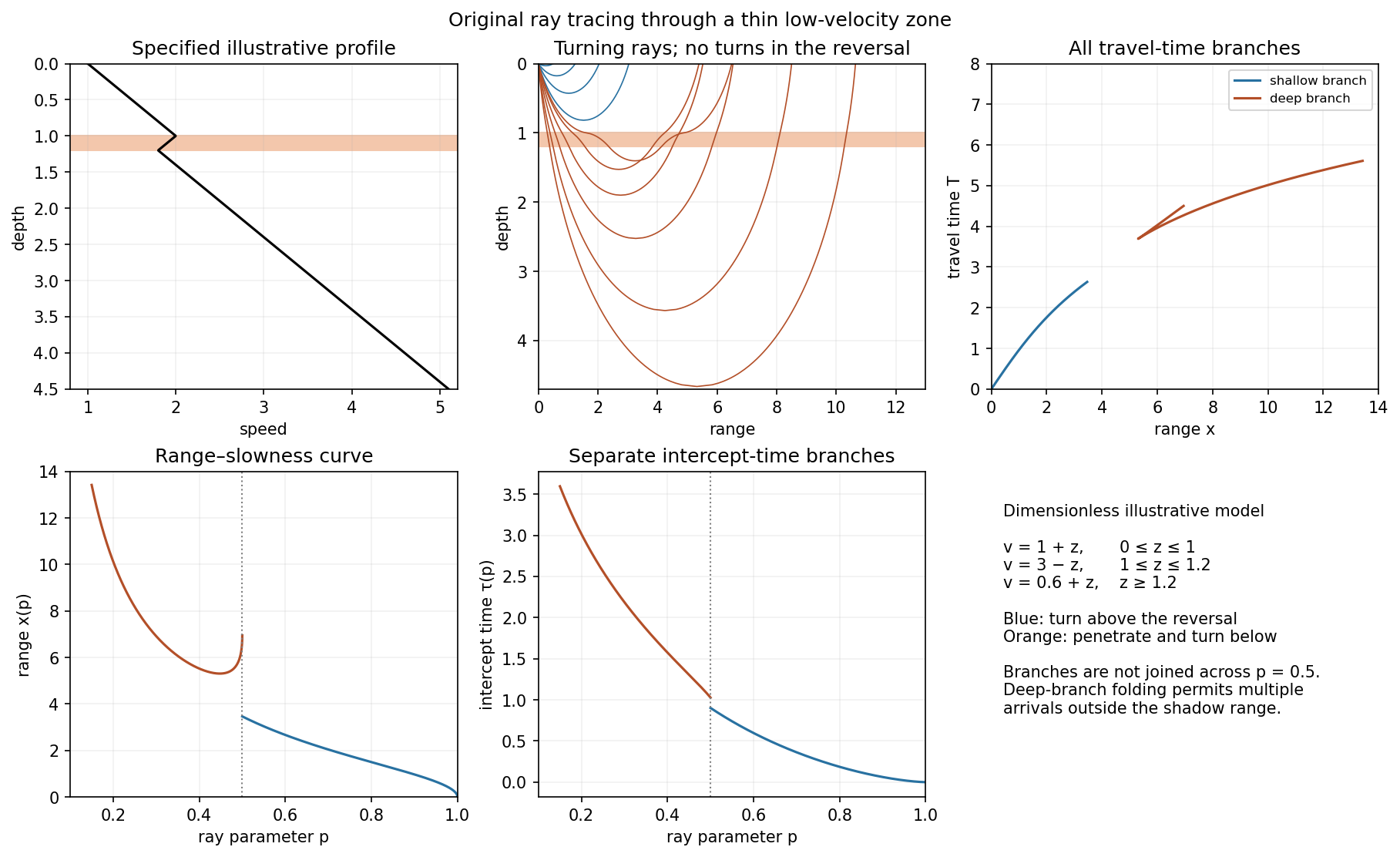
Analytically traced illustrative velocity reversal: rays, travel times, range–slowness and intercept time
. Details. 
Oceanic thermal subsidence. Newly formed oceanic lithosphere is hot and buoyant. Cooling increases its column density, causing subsidence by isostasy as it moves away from a ridge. The half-space cooling model has profile isWith volumetric thermal expansion coefficient , the excess column mass relative to hot mantle isCompensation with seawater density givesThus young-to-intermediate-age seafloor generally deepens approximately as the square root of age. At old ages, finite thermal-plate thickness and basal heat supply flatten this trend; indefinite half-space deepening is inappropriate. Sediments, variable crust, volcanic swells and dynamic topography also perturb bathymetry. Ocean-floor depth and heat flow jointly constrain cooling models.[ref]
An analysis of the variation of ocean floor bathymetry and heat flow with age by Barry Parsons and John G. Sclater. 1977, half-space cooling, bathymetric age trend and finite-plate alternative
Effective elastic thickness. This is the thickness of a homogeneous elastic plate with the observed effective flexural rigidity, not necessarily the crustal or thermal lithospheric thickness:Infer it by modelling deflection around known loads, such as seamounts or trenches, or fitting gravity-topography admittance and gravity-topography coherence across wavelengths. A simple Fourier balance is for a signed transverse load. The transition from buoyancy-dominated to bending-dominated behaviour constrains ; then assumed Young's modulus and Poisson's ratio give .
Good inference includes load geometry and density, buried interfaces, sediment and internal loading, boundary conditions and data resolution. These can trade off with rigidity. Plastic yielding, faulting, mechanical layering and creep make an effective, timescale- and stress-dependent quantity. Older, colder lithosphere is often stronger, but age at loading and subsequent relaxation matter; a single universal age-to- conversion is unjustified.
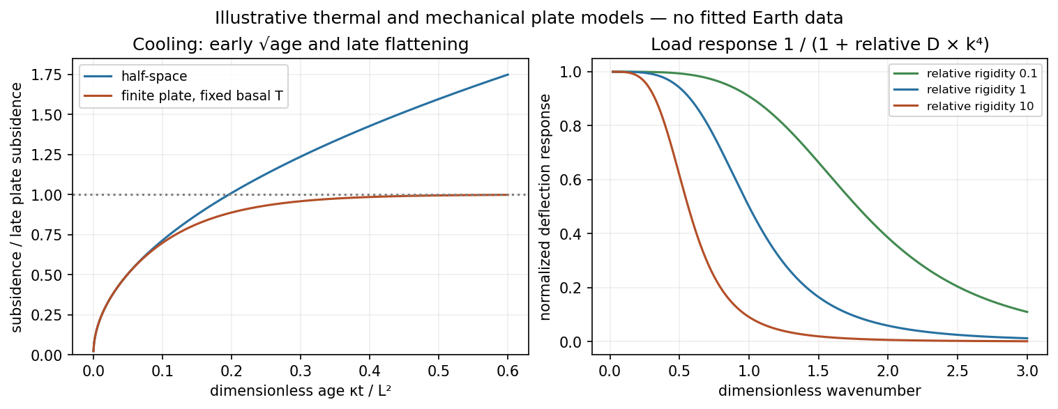
Square-root cooling versus finite-plate saturation, and stiffness sensitivity of the flexural response
. Details. 
Articles by others on the same topic
There are currently no matching articles.