Past exam of the short options paper shared by Prelims and Parts A and B of the physics course of the University of Oxford / 2015 / S3 / 1

The one-dimensional Time-dependent Schrödinger equation isThe left side generates time evolution; the two terms on the right are the kinetic and potential parts of the Hamiltonian operator. For a time-independent potential and an energy eigenstate, set $\psi (x,t)=\varphi (x)e^{-iEt/\hslash }$. Cancelling the time factor gives the time-independent Schrödinger equation, $-{\hslash }^2{\varphi }^{\prime \prime }/(2m)+V\varphi =E\varphi$.

By the Born rule, $|\psi {|}^{2}dx$ is the position probability in an interval of width $dx$, with $\int |\psi {|}^{2}dx=1$ for a normalized particle. Therefore $\boxed{[\psi ]={\mathrm{length}}^{-1/2}}$ in one dimension. An ideal scattering plane wave instead uses flux normalization and is not itself a normalizable single-particle state on the whole line.

The reflection-one result describes a semi-infinite potential step, rather than a finite-width barrier. Define $k=\sqrt{2mE}/\hslash$ and $\kappa =\sqrt{2m(V_0-E)}/\hslash$. For $E>0$, takeThe growing exponential is excluded by boundedness as $x\to \infty$. Continuity of $\varphi$ and ${\varphi }^{\prime }$ at the finite step gives $1+r=c$ and $ik(1-r)=-\kappa c$, henceThe probability current of the decaying tail is zero; the reflected and incident currents have equal magnitude. This agrees with the classical reflection coefficient even though the spatial wave function differs from a classical trajectory.

On the incident side, $\varphi$ is the superposition of incoming and reflected waves, producing a standing-wave pattern whose travelling-wave de Broglie wavelength is $\lambda =2\pi /k$. On the forbidden side, it decays exponentially and remains nonzero near the boundary. A sketch should therefore show oscillations for $x<0$, a continuous function and slope at zero, and the evanescent tail for $x>0$ beside the potential step.

The quantum distinction is finite probability density inside the classically forbidden region, despite complete reflection. There is no transmitted flux at arbitrarily large positive $x$ for this semi-infinite step. A finite-width barrier would allow quantum tunnelling, a different boundary-value problem.

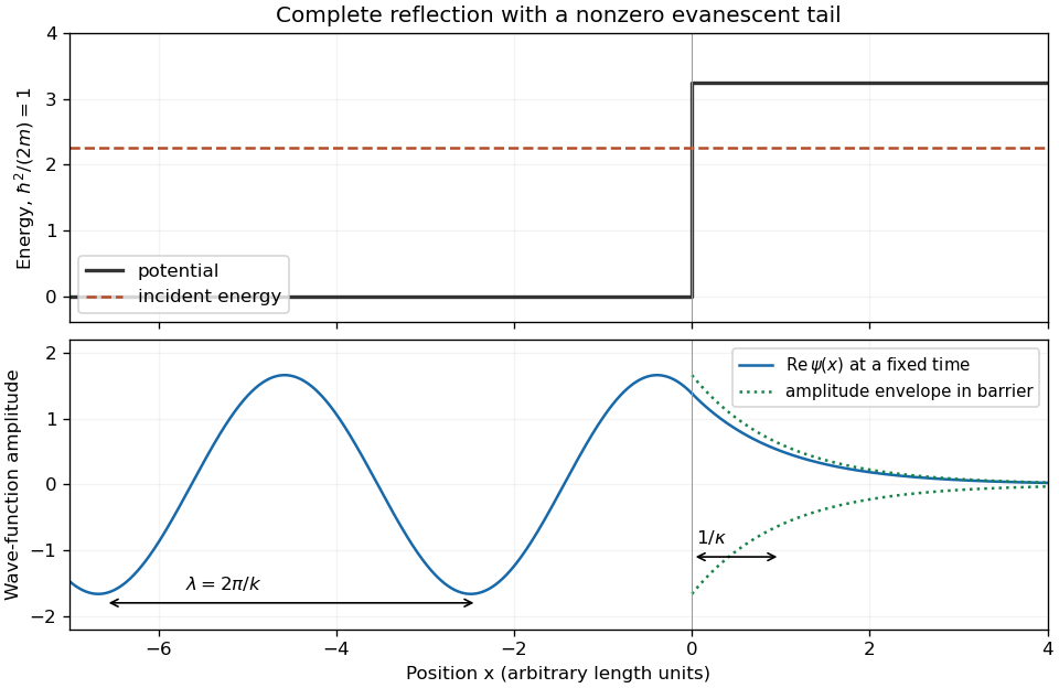
The wave-function amplitude decays as $e^{-\kappa x}$, so its e-folding penetration depth isThe probability density decays as $e^{-2\kappa x}$ and has the smaller e-folding depth $1/(2\kappa )$. Specifying which quantity decays avoids a factor-of-two ambiguity in the term penetration depth.

A stationary evanescent wave does not assign a classical trajectory or a real local speed inside the forbidden region. The dwell time in a semi-infinite potential step measures probability stored in $x>0$ divided by incident probability current. For incident amplitude one,This gives a time in terms of $m,E,V_0$ through the definitions of $k,\kappa$. A simpler dimensional estimate is the penetration length divided by the incident speed, $\Delta x/v_{\mathrm{in}}=m/(\hslash k\kappa )=\hslash /[2\sqrt{E(V_0-E)}]$. The dwell time equals $(2E/V_0)$ times that estimate. Different operational timing definitions need not agree; treating the imaginary under-barrier momentum as a real particle velocity would not justify a unique traversal time.