Treat

X \geq 0

as a prescribed input protein concentration, and

Y (t), Z (t) \geq 0

as the downstream gene-product concentrations. Define the Hill activation function

h (u; K, n) = \frac{u ^{n}}{K ^{n} + u ^{n}}, K > 0, n > 0.

(1)

A minimal model with no basal expression is

\frac{d Y}{d t} = a_{Y} h (X; K_{X Y}, n_{X Y}) - Y, \frac{d Z}{d t} = a_{Z} h (X; K_{XZ}, n_{XZ}) - Z .

(2)

Here

a_{Y}, a_{Z} > 0

are maximal production rates,

K_{X Y}, K_{XZ}

are Hill constants with the same units as

X

, and

n_{X Y}, n_{XZ}

are dimensionless Hill coefficients. The negative terms describe a first-order reaction for loss of each gene product, with both rate constants set to one in the chosen time units. Thus

a_{Y}, a_{Z}

have units of concentration per time and the unit loss rates have units of inverse time.

The equations model regulation of gene expression at the level of its effective protein output, without separate messenger RNA dynamics. The independent branches mean that neither

Y

nor

Z

regulates the other in this initial model. Additive basal production could be included, but is not required by the question and is set to zero throughout this example.

Solution

 0  0

For a constant

X

, set both ordinary differential equation derivatives to zero:

Y^{*} (X) = a_{Y} \frac{X ^{n_{X Y}}}{K _{X Y}^{n_{X Y}} + X ^{n_{X Y}}}, Z_{direct}^{*} (X) = a_{Z} \frac{X ^{n_{XZ}}}{K _{XZ}^{n_{XZ}} + X ^{n_{XZ}}} .

(1)

These equilibrium concentrations are unique for each input. For a loss rate

γ

other than one, divide the corresponding production term by

γ

Choose

a_{Y} = 2

K_{X Y} = 1

n_{X Y} = 2

and

a_{Z} = 3

K_{XZ} = 2

n_{XZ} = 4

. The following Python code plots the requested equilibrium concentrations and defines the functions used in part (c):

import numpy as np
import matplotlib.pyplot as plt

def hill(u, K, n):
    u = np.asarray(u)
    return u**n / (K**n + u**n)

X_grid = np.linspace(0, 5, 501)
Y_eq = 2 * hill(X_grid, 1, 2)
Z_eq = 3 * hill(X_grid, 2, 4)
plt.figure(figsize=(6, 4))
plt.plot(X_grid, Y_eq, label="Y equilibrium: K=1, n=2")
plt.plot(X_grid, Z_eq, label="Z equilibrium: K=2, n=4")
plt.xlabel("X concentration")
plt.ylabel("Equilibrium concentration")
plt.legend()
plt.tight_layout()
plt.show()

The Hill constant sets the half-maximum input:

Y^{*} (1) = 1

and

Z_{direct}^{*} (2) = 1.5

. Increasing that constant shifts activation toward larger

X

. The Hill coefficient changes steepness rather than the half-maximum position; the normalized slope at

X = K

n / (4 K)

. Because the two examples also differ in

K

and maximal production, compare normalized responses when isolating the effect of

n

alone. Both curves vanish at zero and saturate toward their respective maxima.

Figure 1.
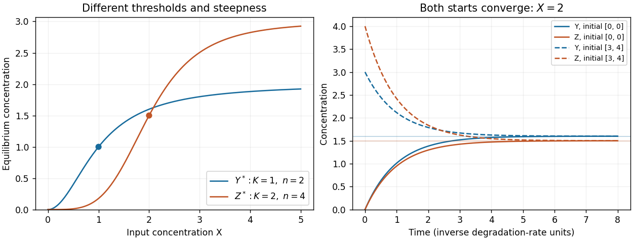
Independent Hill activation and convergence from two initial states
. The left panel shows different half-activation inputs and Hill coefficients. The right panel integrates the two independent output equations at fixed X=2; dashed curves start above equilibrium and solid curves start at zero. **Details**.

Solution

 0  0

At a fixed input the production terms are constant, so both linear ordinary differential equations can also be solved exactly:

Y (t) = Y^{*} + [Y (0) - Y^{*}] e^{- t}, Z (t) = Z_{direct}^{*} + [Z (0) - Z_{direct}^{*}] e^{- t} .

(1)

Each displacement from its equilibrium concentration decays with time constant one. The Jacobian matrix is

- I

, with two eigenvalues equal to

- 1

, so the fixed point is globally asymptotically stable for the nonnegative state space.

Here is a numerical solver using the classical fourth-order Runge-Kutta method; it uses only the repository's existing NumPy and matplotlib dependencies. Continue the definitions from part (b):

def integrate(rhs, initial, times):
    out = np.empty((len(times), len(initial)))
    out[0] = initial
    for j, dt in enumerate(np.diff(times)):
        state = out[j]
        k1 = rhs(state)
        k2 = rhs(state + dt*k1/2)
        k3 = rhs(state + dt*k2/2)
        k4 = rhs(state + dt*k3)
        out[j+1] = state + dt*(k1 + 2*k2 + 2*k3 + k4)/6
    return out

def direct_rhs(state, X):
    Y, Z = state
    return np.array([2*hill(X, 1, 2) - Y,
                     3*hill(X, 2, 4) - Z])

times = np.linspace(0, 8, 801)
plt.figure(figsize=(7, 4))
for initial, style in [([0, 0], "-"), ([3, 4], "--")]:
    trajectory = integrate(lambda s: direct_rhs(s, 2), initial, times)
    exact = np.array([1.6, 1.5]) + (np.array(initial) - [1.6, 1.5]) \
            * np.exp(-times[:, None])
    assert np.max(np.abs(trajectory - exact)) < 1e-8
    plt.plot(times, trajectory[:, 0], style, label=f"Y, initial {initial}")
    plt.plot(times, trajectory[:, 1], style, label=f"Z, initial {initial}")
plt.xlabel("Time")
plt.ylabel("Concentration")
plt.legend()
plt.tight_layout()
plt.show()

For

X = 2

, $Y^{*} = 1.6, Z_{direct}^{*} = 1.5$ . The initial state

(0, 0)

approaches those values from below, while

(3, 4)

approaches from above. Over eight time units the initial displacement is reduced by

e^{- 8} \approx 0.000335

, explaining why both trajectories nearly coincide with the equilibria from part (b). The two-panel figure above displays these simulations.

Solution

 0  0

Add the activating link from

Y

Z

and multiply the two Hill activation functions for the target:

\frac{d Y}{d t} = a_{Y} h (X; K_{X Y}, n_{X Y}) - Y, \frac{d Z}{d t} = a_{Z} h (X; K_{XZ}, n_{XZ}) h (Y; K_{Y Z}, n_{Y Z}) - Z .

(1)

The extra Hill constant

K_{Y Z} > 0

has units of

Y

concentration and

n_{Y Z} > 0

is its Hill coefficient. Both inputs are required for substantial target production: if either is zero, the production term for

Z

vanishes. This all-activating circuit is a coherent feed-forward loop. A product of graded input functions implements the specified AND rule; it is a phenomenological rule rather than a complete molecular promoter model.

Retain the parameter values of parts (b) and (c), and set

K_{Y Z} = 1

n_{Y Z} = 4

. Continue the same Python script with the altered right-hand side:

def and_rhs(state, X):
    Y, Z = state
    return np.array([2*hill(X, 1, 2) - Y,
                     3*hill(X, 2, 4)*hill(Y, 1, 4) - Z])

times = np.linspace(0, 10, 1001)
plt.figure(figsize=(7, 4))
for X in [1, 3]:
    trajectory = integrate(lambda s: and_rhs(s, X), [0, 0], times)
    plt.plot(times, trajectory[:, 0], "--", label=f"Y, X={X}")
    plt.plot(times, trajectory[:, 1], label=f"Z, X={X}")
plt.xlabel("Time")
plt.ylabel("Concentration")
plt.legend()
plt.tight_layout()
plt.show()

X = 1

Y^{*} = 1

and

Z^{*} = (3/17) (1/2) = 3/34 \approx 0.08824

. At

X = 3

Y^{*} = 1.8

and

Z^{*} \approx 2.2873

. In both simulations

Y

first accumulates and opens the additional gate;

Z

therefore initially grows more slowly than under direct activation alone. The equilibrium concentration of

Y

is unchanged by the added outgoing interaction.

Figure 1.
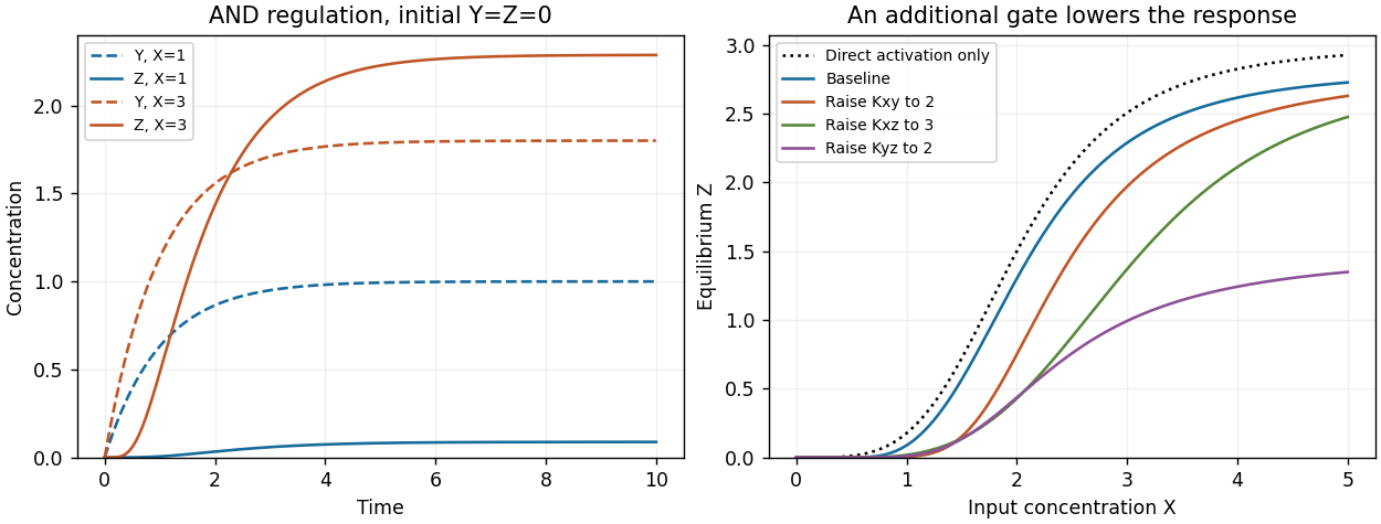
AND feed-forward dynamics and the effect of activation thresholds
. The left panel compares fixed inputs X=1 and X=3 from the zero state. The right panel compares the full feed-forward equilibrium response with direct activation alone and with individual Hill constants increased. **Details**.

e

 0  0

Solution

 0  0

The quasi-steady-state approximation for

Y

sets

Y = a_{Y} h (X; K_{X Y}, n_{X Y})

. Substituting into the

Z

equation gives

\frac{d Z}{d t} = a_{Z} h (X; K_{XZ}, n_{XZ}) h (a_{Y} h (X; K_{X Y}, n_{X Y}); K_{Y Z}, n_{Y Z}) - Z .

(1)

Its equilibrium concentration is therefore

Z_{AND}^{*} (X) = a_{Z} \frac{X ^{n_{XZ}}}{K _{XZ}^{n_{XZ}} + X ^{n_{XZ}}} \frac{( a _{Y} X ^{n_{X Y}} / ( K _{X Y}^{n_{X Y}} + X ^{n_{X Y}} ) ) ^{n_{Y Z}}}{K _{Y Z}^{n_{Y Z}} + ( a _{Y} X ^{n_{X Y}} / ( K _{X Y}^{n_{X Y}} + X ^{n_{X Y}} ) ) ^{n_{Y Z}}} .

(2)

For constant input this is also the exact equilibrium of the full two-variable model: the fast-

Y

assumption is needed to replace the transient dynamics, not to calculate a fixed point.

Relative to the direct-activation result, $Z_{AND}^{*} = Z_{direct}^{*} h (Y^{*}; K_{Y Z}, n_{Y Z}) \leq Z_{direct}^{*}$ . The extra activation gate suppresses the response at low input and can sharpen its rise. The high-input limit is

a_{Z} h (a_{Y}; K_{Y Z}, n_{Y Z})

, which need not reach

a_{Z}

because

Y^{*}

saturates at

a_{Y}

For the parameters in part (d), the following Python continuation plots the expression and changes each Hill constant separately:

def z_equilibrium(X, Kxy=1, Kxz=2, Kyz=1):
    Yeq = 2 * hill(X, Kxy, 2)
    return 3 * hill(X, Kxz, 4) * hill(Yeq, Kyz, 4)

X_grid = np.linspace(0, 5, 501)
plt.figure(figsize=(7, 4))
plt.plot(X_grid, 3*hill(X_grid, 2, 4), ":", label="Direct activation")
for parameters, label in [((1, 2, 1), "Baseline"),
                          ((2, 2, 1), "Kxy=2"),
                          ((1, 3, 1), "Kxz=3"),
                          ((1, 2, 2), "Kyz=2")]:
    plt.plot(X_grid, z_equilibrium(X_grid, *parameters), label=label)
plt.xlabel("X concentration")
plt.ylabel("Equilibrium Z")
plt.legend()
plt.tight_layout()
plt.show()

Increasing

K_{X Y}

lowers

Y^{*}

at fixed finite

X

, delaying opening of the indirect gate. Increasing

K_{XZ}

delays opening of the direct gate. Neither changes the limiting response as

X \to \infty

, provided the constants remain finite. Increasing

K_{Y Z}

makes a given

Y

less effective and also lowers the high-input plateau. These changes are visible in the preceding figure. At small

X

, the response is proportional to

X^{n_{XZ} + n_{X Y} n_{Y Z}}

, while both gates are far below saturation, explaining the increased low-input suppression.

For a persistence detector, retain finite

Y

dynamics and use, for example,

a_{Y} = a_{Z} = 1, K_{X Y} = K_{XZ} = 1, n_{X Y} = n_{XZ} = 4, K_{Y Z} = 0.7, n_{Y Z} = 8,

(3)

with unit loss rates,

X_{off} = 0

X_{on} = 2

, and initially

Y = Z = 0

. On switching the input on,

Y_{\infty} = 16/17

and

Y (t) = \frac{16}{17} (1 - e^{- t}) .

(4)

The time to reach the half-activation threshold of the indirect gate is

t_{gate} = - lo g (1 - \frac{0.7}{16/17}) = lo g (160/41) \approx 1.362 .

(5)

An isolated input pulse of duration

0.25

ends well before this threshold; a duration-four pulse persists long enough to open the gate. The large but finite Hill coefficient makes this a graded filter, not a perfectly sharp cutoff. Once

X

vanishes, its direct gate closes immediately and stops production of

Z

, which then decays with time constant one. The protein output itself does not drop discontinuously. This delayed-on, prompt-production-off mechanism is the characteristic persistence detector interpretation of an AND-type coherent feed-forward loop.^[ref]

This final Python continuation simulates both pulse durations. Each discontinuity is placed on the time grid and the input is held constant within each integration step:

def persistence_rhs(state, X):
    Y, Z = state
    return np.array([hill(X, 1, 4) - Y,
                     hill(X, 1, 4)*hill(Y, 0.7, 8) - Z])

def pulse_trajectory(duration, dt=0.005):
    times = np.arange(round(8/dt) + 1) * dt
    out = np.zeros((len(times), 2))
    for j in range(len(times)-1):
        X = 2.0 if 1 <= times[j] + dt/2 < 1 + duration else 0.0
        # Each step is integrated with its constant input.
        out[j+1] = integrate(lambda s: persistence_rhs(s, X),
                             out[j], [0, dt])[-1]
    return times, out

fig, axes = plt.subplots(1, 2, figsize=(10, 4))
for duration in [0.25, 4]:
    times, out = pulse_trajectory(duration)
    axes[0].plot(times, out[:, 0], label=f"Y, duration {duration}")
    axes[1].plot(times, out[:, 1], label=f"Z, duration {duration}")
    print(duration, "maximum output", out[:, 1].max())
axes[0].axhline(0.7, color="black", linestyle=":")
for ax in axes:
    ax.set_xlabel("Time")
    ax.set_ylabel("Concentration")
    ax.legend()
plt.tight_layout()
plt.show()

The chosen example produces peak

Z

of about

1.72 \times 1 0^{- 6}

for the short pulse and

0.766

for the long pulse. These are original illustrative simulations, not fitted experimental measurements.

Figure 1.
A coherent feed-forward loop distinguishes short and persistent input pulses
. Both inputs switch from zero to X=2 at time one. One ends after 0.25 time units and the other after four. The intermediate Y crosses its activation threshold only for the sustained input, producing a much larger target response. **Details**.

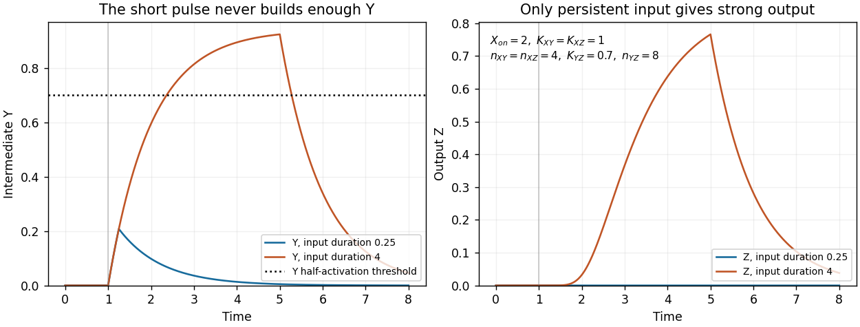
Finally, the strict instantaneous-

Y

reduction used for the equilibrium calculation has no separate intermediate accumulation delay. Its remaining one-variable dynamics can still attenuate short pulses through ordinary output relaxation, but it cannot demonstrate the additional delay caused by finite

Y

buildup. The pulse test therefore uses the full two-variable model.

Past exam of the systems biology course of the University of Cambridge / 2024 / Paper 3 / 3

a

Solution

b

Solution

c

Solution

d

Solution

e

Solution

 Ancestors (11)

 Discussion (0)

 Articles by others on the same topic (0)

Past exam of the systems biology course of the University of Cambridge / 2024 / Paper 3 / 3

 Discussion (0)  Subscribe (1)

 Discussion (0)