Past exam of the year 2 of the earth sciences (geology) course of the University of Oxford / 2024 / Paper 3 / 3

Use compression-positive principal stresses, ${\sigma }_1\ge {\sigma }_2\ge {\sigma }_3$. For the intended thrust fault regime during approximately north–south tectonic shortening, the likely orientations areA locally horizontal traction-free surface motivates taking one principal direction as vertical, while the strong north–south compression selects the maximum horizontal principal stress. The expected fault strike is then approximately east–west.

This ordering assumes the two horizontal compressions exceed the vertical principal stress. North–south shortening by itself does not establish the magnitudes of all three: if the vertical principal stress were intermediate, strike-slip faulting would instead be possible. The answer above is the simple compressional end member used in the following parts.

A reverse or thrust fault earthquake is the expected end member: a hanging wall moves upwards relative to its footwall, accommodating north–south tectonic shortening. A plausible double-couple seismic source focal mechanism has an approximately east–west fault strike, a moderately north- or south-dipping fault plane, and up-dip fault slip. For example, right-hand-rule strike $090^{\circ }$, southward fault dip about $32^{\circ }$, and fault rake $+90^{\circ }$ specify a pure thrust mechanism.

In a lower-hemisphere equal-area plot, with shaded regions denoting compressional P first motions, this focal mechanism has a shaded central region and two unshaded outer lobes. The P axis is approximately horizontal north–south and the T axis approximately vertical for a symmetric idealization; for a single $32^{\circ }$ plane their axes are slightly tilted. The P and T axes of a double-couple seismic source need not exactly equal the regional principal stress axes. The nodal curves represent both the fault plane and its auxiliary plane; additional evidence is needed to choose between them.^[ref]

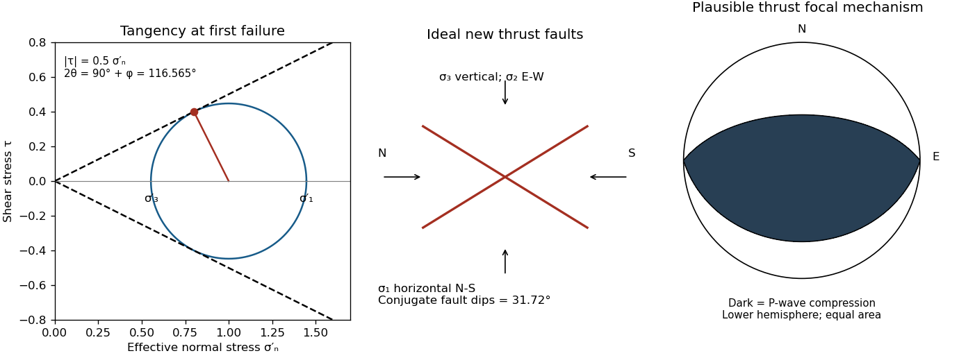
Assume an initially unfractured homogeneous isotropic material described by a linear Mohr-Coulomb failure criterion, with the given coefficient of friction ${\mu }_f=0.5$ representing the relevant internal friction angle. Use spatially uniform pore fluid pressure, effective stresses ${\sigma }_i^{\prime }={\sigma }_i-P_f$, and compression-positive signs. ThenThe Mohr circle in the ${\sigma }_1^{\prime },{\sigma }_3^{\prime }$ plane has centre $C=({\sigma }_1^{\prime }+{\sigma }_3^{\prime })/2$ and radius $R=({\sigma }_1^{\prime }-{\sigma }_3^{\prime })/2$. At first failure it is tangent to the failure envelope. The radius to the positive-shear tangent point is perpendicular to the line of slope $\tan \phi$, hence makes angle $90^{\circ }+\phi$ with the positive normal-stress axis.

If $\theta$ is the angle between the fault normal and ${\sigma }_1$, the stress transformation isThus $2\theta =90^{\circ }+\phi$, $\theta =58.2825^{\circ }$, and the angle of the fault itself to horizontal ${\sigma }_1$ isThe two conjugate thrust faults therefore strike approximately east–west and dip about $32^{\circ }$ north and $32^{\circ }$ south. This is the fault dip, not the $58.3^{\circ }$ fault-normal angle. Both sediments and basement have the same optimum orientation under these assumptions because their stipulated friction slopes are equal; their cohesion and absolute failure stresses could still differ.

The first two panels in solution give the labeled construction. Constant cohesion shifts the straight failure envelope without changing its slope, and uniform pore fluid pressure translates the Mohr circle in normal-stress coordinates; neither changes this tangency angle. In the illustrative cohesionless case, $R/C=\sin \phi$, giving ${\sigma }_1^{\prime }/{\sigma }_3^{\prime }=(1+\sin \phi )/(1-\sin \phi )\simeq 2.618$. Pre-existing weaknesses, a nonuniform stress field, anisotropic strength, or a nonlinear failure envelope invalidate the simple optimum-orientation prediction.^[ref]

The $31.7^{\circ }$ result predicts initial failure in a uniform material under the assumed principal-stress orientations. The actual Figure 3 is a present-day NW–SE cross section through a thick, heterogeneous Alpine stack, extending to about 50 km depth. It contains near-horizontal basal stretches, curved ramps, tightly bent contacts, and steep structures in the internal zones around Viso and the Dora Maira complex. It does not show a single undeformed conjugate pair newly formed in horizontal uniform rock.

Several processes explain the departures:

Finally, a section shows apparent dip unless it is perpendicular to fault strike. For an ideal plane, $\tan {\delta }_{\mathrm{app}}=\tan {\delta }_{\mathrm{true}}\sin \alpha$, where $\alpha$ is the angle between the section direction and fault strike. Obliquity can make a plane look shallower, but cannot on its own explain an apparent dip steeper than its true dip. Do not infer that each black curve is a currently active brittle earthquake fault.

The northern station is closer, under comparable P wave and S wave paths through the same velocity model. In the actual Figure 4 the northern P and S pulses are separated by about 6 s, whereas the southern separation is roughly 8–8.5 s. The S–P time removes the unknown earthquake origin time:Both northern pulses also occur earlier on the shared absolute clock, consistent with the smaller distance. Earlier arrival alone would not be sufficient if clocks or velocity models differed.

For reproducible graph readings, the northern positive-to-negative zero crossings are approximately $13.3\mathrm{s}$ for P and $19.3\mathrm{s}$ for S; the southern crossings are approximately $16.7\mathrm{s}$ and $25.0\mathrm{s}$. These are convenient corresponding pulse landmarks, not sharply defined first-break onsets. The first visible motion begins earlier: approximately 12 s and 18 s in the north, and 14–15 s and 22–23 s in the south, depending on the amplitude threshold. The horizontal axis is seconds since midnight on 1 January 2000, not elapsed time since rupture initiation.

Use the northern S–P time, approximately $\Delta t_N=6\mathrm{s}$, rather than multiplying an absolute-clock arrival by a wave speed. For common approximately straight paths,No numerical crustal velocities are specified in Q3. If the usual illustrative crustal values $V_p=6.0\mathrm{km}{\mathrm{s}}^{-1}$ and $V_s=3.5\mathrm{km}{\mathrm{s}}^{-1}$ are adopted, the distance isThese assumed crustal speeds are unrelated to Q1's offshore layer values. They are representative rather than measurements of the Swiss column; the British Geological Survey gives broad typical crustal ranges of 5–7 km/s for P waves and 3–4 km/s for S waves.^[ref]

Using the corresponding northern central pulse times gives an effective source time near $13.3-50.4/6\simeq 4.9\mathrm{s}$ after midnight, and the S estimate is the same to graph accuracy. The southern central landmarks similarly give a distance near 70 km and an effective source time near 5 s. That consistency supports the example, but pulse landmarks need not mark the rupture's true onset. $D_N$ is a source-to-station path or hypocentral distance in the uniform-speed approximation. An epicentral distance additionally needs the hypocenter depth; it cannot simply be equated to 50 km for an unknown depth.

Distinguish the duration of one phase pulse from the P-to-S separation. Figure 4 shows northern pulses with most visible motion over roughly 3–4 s each, compared with roughly 4–5 s or more in the south. Reading the low-amplitude tails gives approximately 11.5–15.2 s for the northern P pulse, 17.7–20.9 s for the northern S pulse, 14.2–19.0 s for the southern P pulse, and 22.3 s to beyond the right plot boundary near 27 s for the southern S pulse. Thus the latter duration is censored by the plotting window; it should not be assigned an exact ending at 27 s. The positive-to-negative extremum separations are only about 1 s in the northern pulses, 1.3 s in the southern P pulse and 1.4 s in the southern S pulse; those much shorter numbers are not full source durations. Smooth tails have no unique onset or ending at the precision of this drawing.

A finite-source rupture has an intrinsic duration $T$ that differs from the apparent pulse duration through rupture directivity. In an ideal unilateral line-source model, neglecting local slip rise time, instrument filtering and path broadening,Here $c$ is the chosen phase wave speed and $L_{\parallel }$ is the rupture's projection along equal-and-opposite takeoff directions. Averaging corresponding full pulses in that model suggests an intrinsic timescale of roughly 4–5 s. This is an order-of-magnitude graph estimate, not an exact rupture duration; the figure does not supply a seismic source time function definition, receiver responses, phase deconvolution, or geometry sufficient to determine one uniquely. A finite local slip rise time would also contribute to the observed width.

In particular, neither 13 s nor 19 s is a rupture duration: those numbers locate phase motion on the absolute clock. The northern P–S gap of 6 s is a propagation delay rather than the rupture duration.

For a unilateral finite-source rupture advancing at approximately constant rupture velocity $V_r$, the along-fault propagation length isThere is no supplied $V_r$ or calibrated seismic source time function, so a unique spatial extent cannot be read directly from Figure 4. For illustration, $T\sim 4\mathrm{s}$ and an assumed $V_r\sim 2.5\mathrm{km}{\mathrm{s}}^{-1}$ would give $L\sim 10\mathrm{km}$. Allowing $T\sim 4$–$5\mathrm{s}$ and assumed $V_r\sim 2$–$3\mathrm{km}{\mathrm{s}}^{-1}$ gives lengths of order 8–15 km. These are explicitly conditional scale estimates, not measured fault dimensions.

If equal-and-opposite ray geometry and phase pulse durations were known, the directivity model in solution would instead constrain a projected length,where $\psi$ is the angle between the rupture direction and the northern ray. Distinct P and S wave speeds, unknown takeoff angles, smooth pulse boundaries and the clipped southern S tail prevent a reliable independent numerical inversion here. This observation is consistent with a few-kilometre projected extent while the actual along-fault length can be larger. A rupture length is not the accumulated fault slip, the width of the whole fault plane, or the approximately 50 km station distance.

The shorter, stronger northern pulses and broader southern pulses suggest propagation from south to north, towards the northern station. The useful evidence is the difference in pulse widths, not just the earlier northern arrivals: the latter chiefly reflect station distance.

As rupture reaches successively more northerly patches, each patch radiates a new P wave and S wave pulse. Towards the north, the later emission time is partly cancelled by a shorter propagation path; those contributions arrive closer together. Towards the south, later emission and a longer path add, stretching the signal. This is rupture directivity. It refers to the advance of the slipping region along the fault, not necessarily the direction of the local fault slip vector. A thrust can slip up-dip while its rupture front advances in a direction with a northward component.

More generally, emission from a patch at distance $s$ along the rupture arrives atThe forward direction has a smaller arrival-time spread. This is the same travel-time compression captured by isochrone-based rupture directivity calculations.^[ref] Larger northern amplitude supports the interpretation but is not decisive on its own because geometrical spreading, seismic attenuation, seismic radiation patterns and site response also affect amplitude. With only two traces, propagation, filtering and site effects remain alternatives to test; the idealized exercise is most naturally explained by northward directivity.