Past exam of the year 2 of the earth sciences (geology) course of the University of Oxford / 2024 / Paper 3 / 8

The consistent matching is:

Series C stops after about six months, identifying machine 2. Its short record gives spectrum W a coarser Fourier frequency resolution. Series A resolves the annual variation but misses the changing daily phase: the regular three-day interval samples the daily oscillation at the same phase, so its daily contribution aliases to a constant. Its spectrum is Y. Machine 3 produces the half-daily-frequency alias in X, leaving D as its time series. The fully sampled two-year record B and spectrum Z agree with the supplied first row.

These identifications use the record lengths, frequency locations and sampling intervals. They do not require assuming that the plotted spectral heights have an identical normalization.

Sixteen hours is $2/3$ of a day, so the sampling rate is

The conventional Nyquist frequency isFrequencies above this cutoff are indistinguishable from lower-frequency sampled sinusoid aliases. The Nyquist–Shannon sampling theorem requires a band limit strictly below the cutoff for general phase information: at exactly the cutoff, some phases can give zero samples. Thus $32$ hours is the conventional limiting period, with unambiguous reconstruction requiring a longer period under those sampling assumptions.

The true daily component has $f_D=1\mathrm{da}{\mathrm{y}}^{-1}$, above machine 3's Nyquist frequency. At sampling times $t_n=2n/3$ days,The last sequence is also produced by a continuous cosine with frequency $0.5\mathrm{da}{\mathrm{y}}^{-1}$ sampled at those same times. Hence the observed peak is the sampled sinusoid aliasIt is not evidence for an additional two-day physical temperature cycle.

The source text and its figure are inconsistent here. The plotted low-frequency maximum in W is near $0.0055\mathrm{da}{\mathrm{y}}^{-1}$, rather than the printed $0.055\mathrm{da}{\mathrm{y}}^{-1}$. The original PDF shows that this discrepancy is already present in the examination, rather than introduced by transcription.

Machine 2 records only about half a year. Its first nonzero discrete Fourier transform bin is therefore atThe annual component near $1/365\mathrm{da}{\mathrm{y}}^{-1}$ is below that first bin. The finite window function spreads it through spectral leakage, with a prominent first-bin contribution. This explains the plotted peak without invoking a new physical period.

A literal peak at $0.055\mathrm{da}{\mathrm{y}}^{-1}$ would instead have a period of about $18.2$ days. Neither the two stated model frequencies nor the given sampling schedule identifies such a separate component. The interpretation above treats the printed decimal as an apparent typo; it does not silently change the stated number.

The adequately sampled record shows a yearly cycle and a daily cycle. Up to exchanging their labels,Using $365$ days per year for numerical estimates,These are angular frequencies. The corresponding ordinary frequencies are $1\mathrm{y}{\mathrm{r}}^{-1}$ and $1\mathrm{da}{\mathrm{y}}^{-1}$.

Write ${\delta }_j=\sqrt{2K/{\omega }_j}$ for each component's thermal penetration depth. Its contribution at depth isThus its amplitude is multiplied by $e^{-x/{\delta }_j}$ and its wave phase lags the surface by $x/{\delta }_j$ radians. The corresponding unwrapped time lag is $x/({\delta }_j{\omega }_j)$; a phase measured from a single periodic signal is observable only modulo $2\pi$.

Higher-frequency variations have smaller penetration depths. In particular,The daily oscillation is therefore strongly attenuated at depths where a substantial annual oscillation survives. This is a thermal diffusion wave, whose phase lag is not the arrival time of a sharp thermal front. The displayed solution is the established periodic response; an additional transient would depend on initial subsurface data not needed for this interpretation.

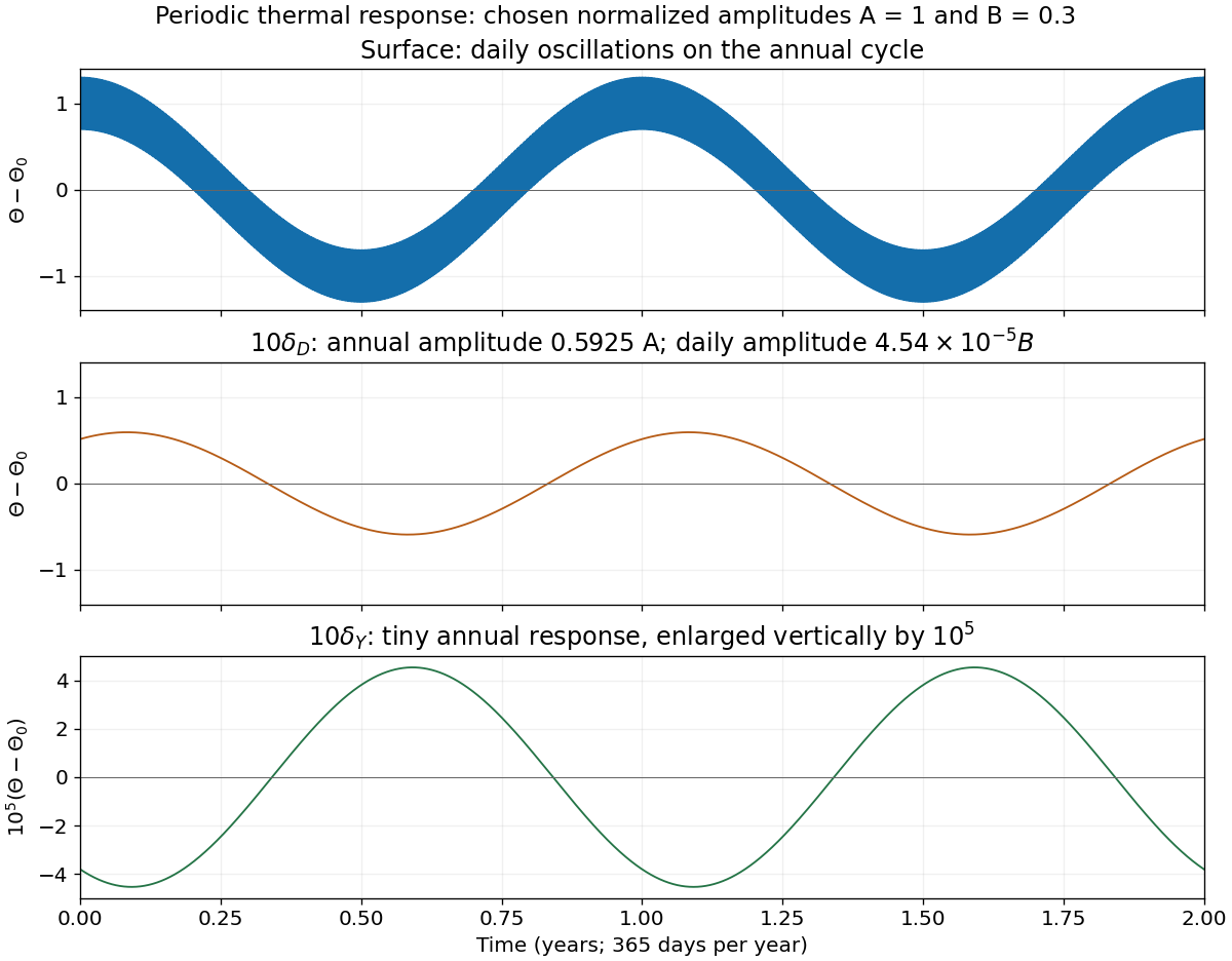
For the sketches, take $A$ to multiply the annual component and $B$ the daily component. Their amplitudes are left as parameters, as in the model.

At the surface both attenuation factors are one and both lags vanish:The sketch is a rapid daily oscillation on a slowly varying annual background. The amplitudes cannot be inferred uniquely from the sampling intervals alone.

At $x=10{\delta }_D$, the daily component is multiplied by $e^{-10}\simeq 4.54\times 10^{-5}$ and has a lag of ten radians. The annual component instead has $x/{\delta }_Y=10/\sqrt{365}\simeq 0.5234$. HenceThe sketch is nearly a smooth annual sinusoid, with annual amplitude about $0.5925A$ and annual phase lag about $0.5234$ radians, corresponding to about $30.4$ days on the chosen year scale. The tiny daily component is retained in the formula rather than declared identically zero.

At $x=10{\delta }_Y$, the annual attenuation is $e^{-10}$ and the daily attenuation is $e^{-10\sqrt{365}}$, approximately $10^{-83}$. ThusOn the same vertical scale as the surface plot this is almost the constant ${\Theta }_0$. With a sufficiently enlarged scale, a residual annual oscillation of amplitude $4.54\times 10^{-5}A$ remains. Its phase lag is ten radians, interpreted modulo $2\pi$ when comparing periodic maxima.