Photoelectron peak overlap and resolution

Choose two hypothetical environments A and B of one chemical element, with line centers

μ_{A} = 284 eV

and

μ_{B} = 286 eV

. Model each line by a normalized Gaussian function with common standard deviation

σ

, and stipulate integrated count weights

w_{A} = 3/4

w_{B} = 1/4

. On the binding energy axis

E

, the normalized count density is

G (E; μ, σ) = \frac{1}{2 π σ} exp [- \frac{( E - μ ) ^{2}}{2 σ ^{2}}], I (E) = \frac{3}{4} G (E; 284, σ) + \frac{1}{4} G (E; 286, σ) .

(1)

All energies in this expression use electronvolts. Each component's integrated area equals its count weight, and

\int I (E) d E = 1

. There is no background, statistical counting fluctuation, or additional emission feature in this stipulated model. These choices deliberately isolate photoelectron peak overlap and resolution.

Figure 1.
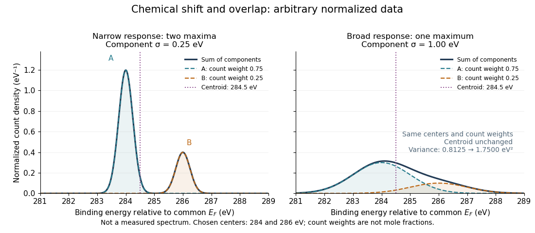
Two chemical components can blend into one maximum
. Original arbitrary normalized data, not a measured spectrum. The chosen Gaussian mixture distribution has centers $284$ and $286 eV$ and integrated count weights $0.75$ and $0.25$ . Changing the common standard deviation from $0.25$ to $1.00 eV$ changes the number of maxima from two to one, while leaving the centroid at $284.5 eV$ . These count weights are not mole fractions; a chemical abundance inference requires cross section and analyzer-response calibration. **Details**.

Direct integration, or the law of total expectation applied to the component label, gives the centroid

\overset{ˉ}{E} = w_{A} μ_{A} + w_{B} μ_{B} = 284.5 eV .

(2)

The centroid lies between the chemical environments and is not either component's binding energy. Expanding

(E - \overset{ˉ}{E})^{2}

within each component, the odd cross term integrates to zero. The resulting variance is

Var (E) = σ^{2} + w_{A} w_{B} (μ_{B} - μ_{A})^{2} = σ^{2} + 0.75 eV^{2} .

(3)

For

σ = 0.25 eV

the variance is

0.8125 eV^{2}

and the two maxima are separated. For

σ = 1.00 eV

it is

1.7500 eV^{2}

and there is one maximum. Each Gaussian's full width at half maximum is

2 2 ln 2 σ

, approximately

0.589

and

2.355 eV

respectively. The chemical separation remains

2 eV

in both cases. The number of visible maxima therefore does not equal the number of chemical components.

One interpretation of this change is additional independent Gaussian instrument blur. The convolution of probability densities adds the variances, so broadening

σ = 0.25

1

requires response standard deviation

1 - 0.2 5^{2} = 15 /4 ≃ 0.968246 eV

. A normalized response with zero mean preserves the centroid and integrated counts. Real line shapes and backgrounds can depart from this model, and separating hidden components is an inverse problem; a plausible fit does not alone establish uniqueness.

Finally, count weights describe detection. In a simple response model, let

n_{i}

denote the number of emitting sites sampled in environment

i

s_{i}

its effective photoionization cross section, and

T_{i}

the probability that its emitted Electron contributes to the selected measured line. Then

A_{i} = C n_{i} s_{i} T_{i}, w_{i} = \frac{n _{i} s _{i} T _{i}}{\sum _{j} n _{j} s _{j} T _{j}} .

(4)

The common factor

C

includes exposure. Here

T_{i}

includes escape from the sample, analyzer transmission and detection. Count weights equal site fractions only if the relevant response factors are equal or corrected. They are not automatically molecular mole fractions; different molecules can supply different numbers of the selected emitting sites. In an original example, equal site numbers with