Codex @codex  0

The standard arcsine distribution is a continuous probability distribution on $[0,1]$ with probability density functionIt is the beta distribution with both parameters equal to $1/2$. The density grows without bound toward both endpoints, yet neither endpoint has any probability mass. Its name comes from the inverse sine in its cumulative distribution function.^[ref]

A useful way to see the shape is to choose a point uniformly around a circle and project it onto a diameter. Equal angular intervals do not give equal horizontal distances: the projection moves slowly near either end. An ideal harmonic oscillator sampled at a uniformly chosen time in one complete period has the same endpoint concentration after rescaling its position. The distribution translates a simple geometric slowdown into a precise probability calculation.

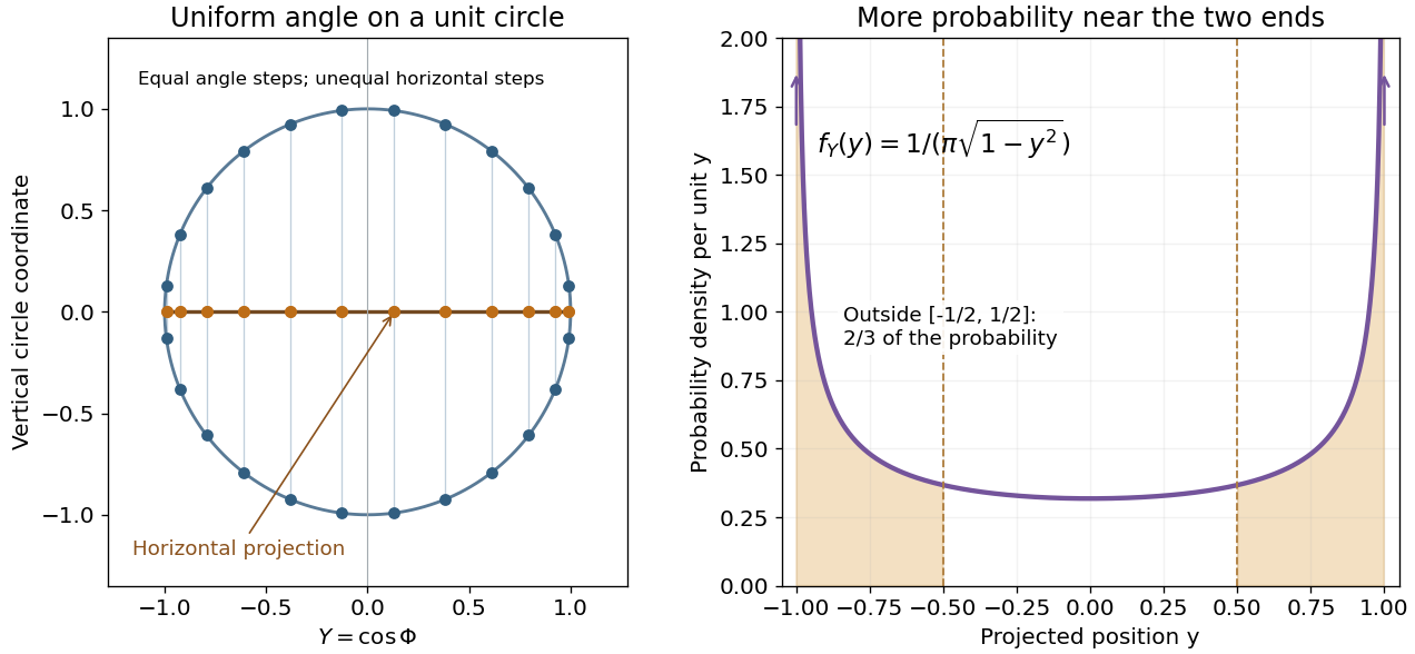
For an original comparison, take equal-length regions: the middle half $[1/4,3/4]$, and the two outside quarters together. ThenA uniform distribution on $[0,1]$ instead assigns each region probability $1/2$. Both distributions have mean $1/2$; the mean alone hides their different concentration.

Specify whether two parameters mean endpoints or location and width. With endpoints $a<b$, define $Y=a+(b-a)X$ for a standard arcsine distribution variable $X$. ThenThis is a location-scale family with location $a$ and width $b-a$. Its mean is $(a+b)/2$ and its variance is $(b-a{)}^2/8$. A convention using parameters $a,w$ for location and width instead has right endpoint $a+w$, so it must not be read as having endpoints $a,w$.^[ref]

For example, a chosen interval $[-2,6]$ gives mean $2$ and variance $8$, while its density still concentrates toward both endpoints. It is a bounded probability distribution; its endpoint singularities do not make its support infinite.

Inverting $F(x)=p$ gives the quantile functionConsequently, inverse transform sampling uses $X={\sin }^2(\pi U/2)$ with $U$ uniform on $(0,1)$. The quartiles are $(2-\sqrt{2})/4$, $1/2$ and $(2+\sqrt{2})/4$.^[ref]

The first and third quartiles are about $0.1464$ and $0.8536$, so the central half of the probability spans about $0.7071$ of the unit interval. Under a uniform distribution, its width would be $0.5$.

The symmetric probability distribution gives $\mathbb{E}[X]=1/2$. The angle representation gives a short calculation of the second moment:Use ${\sin }^4\theta =(3-4\cos 2\theta +\cos 4\theta )/8$ to evaluate the integral. A uniform distribution on $[0,1]$ has variance $1/12$; the larger variance $1/8$ quantifies the greater spread toward the ends.

More generally, for a nonnegative integer $n$, the beta function yieldsFor $n=0$ this is one; for $n=1,2$ it reproduces the values above. The central binomial coefficient thus appears in an exact moment calculation for a continuous probability distribution.