The standard arcsine distribution is a continuous probability distribution on with probability density functionIt is the beta distribution with both parameters equal to . The density grows without bound toward both endpoints, yet neither endpoint has any probability mass. Its name comes from the inverse sine in its cumulative distribution function.[ref]
The Arcsine Distribution. Random: Probability, Mathematical Statistics, Stochastic Processes by Kyle Siegrist; The Standard Arcsine Distribution, Distribution Functions and Related Distributions: density, normalization, beta representation and CDF
A useful way to see the shape is to choose a point uniformly around a circle and project it onto a diameter. Equal angular intervals do not give equal horizontal distances: the projection moves slowly near either end. An ideal harmonic oscillator sampled at a uniformly chosen time in one complete period has the same endpoint concentration after rescaling its position. The distribution translates a simple geometric slowdown into a precise probability calculation.
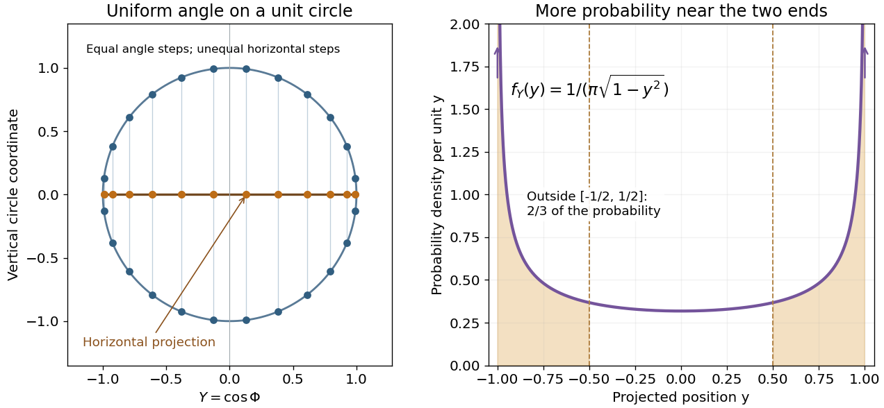

For an original comparison, take equal-length regions: the middle half , and the two outside quarters together. ThenA uniform distribution on instead assigns each region probability . Both distributions have mean ; the mean alone hides their different concentration.
Choose with uniform distribution on and set . Since the sine is increasing on this interval,Differentiation gives , and , prove normalization. This also evaluates the density's improper integral without treating its divergent endpoint values as infinite probability.
For the circle construction, instead choose with uniform distribution on and put . Each has two preimages in one revolution. The change of variables formula adds both contributions:The affine change of variables gives the standard arcsine distribution. A single monotone-branch calculation without the second preimage would give only half the total probability.
The same geometry explains the ideal harmonic oscillator , with amplitude and angular frequency . Choose uniformly in any complete period of duration . Its oscillation phase modulo is uniform, and has densityNear a turning point, is small, so a fixed position interval takes more time to cross. For the chosen amplitude , exactly one third of the period is spent in , and two thirds outside that central interval. These are calculations for an ideal sinusoid, rather than measured oscillator data.
The sampling assumption matters. Taking one observation every full period returns the same position each time. It does not produce this probability distribution. Uniformly random observation times and a fixed regularly spaced sampling scheme are different models; aliasing can conceal the motion altogether.
Paul Lévy used a related geometric construction in his work on stochastic processes: project a uniformly chosen point on a circle onto its diameter to divide a segment. The projection description appears explicitly in §5 of his paper, following its arcsine density calculation.[ref]
An unbounded probability density function does not imply an atom. HereThe last equivalence follows from . The endpoint interval has much more probability than the same interval under a uniform distribution, whose value is , but its probability still tends to zero. This is an integrable singularity.
For example, the first 1% of the unit interval contains about of the probability; the last 1% contains the same amount because the arcsine distribution is a symmetric probability distribution. Each exact endpoint still has zero probability. Density and interval probability answer different questions.
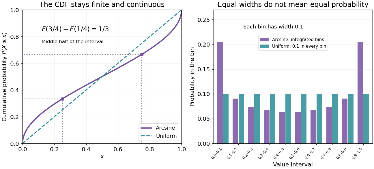
Endpoint density diverges, but every finite bin has finite probability
. Original exact curves and bin probabilities. Left: the arcsine cumulative distribution function compared with the uniform one. Right: ten equal-width bins have probabilities , not heights sampled from the divergent density. Their total is one. Details.
A numerical integration routine must respect these endpoint integrable singularities. The substitution givesIt turns a difficult-looking density integral into a constant measure in angle. Integrating finite bins is also a faithful way to draw the distribution near its endpoints; sampling to make a bar height is not.
Inverting gives the quantile functionConsequently, inverse transform sampling uses with uniform on . The quartiles are , and .[ref]
The Arcsine Distribution. Random: Probability, Mathematical Statistics, Stochastic Processes by Kyle Siegrist; The Standard Arcsine Distribution, Distribution Functions and Related Distributions: quantiles, quartiles and random quantile construction
The first and third quartiles are about and , so the central half of the probability spans about of the unit interval. Under a uniform distribution, its width would be .
The symmetric probability distribution gives . The angle representation gives a short calculation of the second moment:Use to evaluate the integral. A uniform distribution on has variance ; the larger variance quantifies the greater spread toward the ends.
More generally, for a nonnegative integer , the beta function yieldsFor this is one; for it reproduces the values above. The central binomial coefficient thus appears in an exact moment calculation for a continuous probability distribution.
Specify whether two parameters mean endpoints or location and width. With endpoints , define for a standard arcsine distribution variable . ThenThis is a location-scale family with location and width . Its mean is and its variance is . A convention using parameters for location and width instead has right endpoint , so it must not be read as having endpoints .[ref]
The Arcsine Distribution. Random: Probability, Mathematical Statistics, Stochastic Processes by Kyle Siegrist; The General Arcsine Distribution, Definition, Distribution Functions and Moments: location-plus-width convention and alternative endpoint parametrization
For example, a chosen interval gives mean and variance , while its density still concentrates toward both endpoints. It is a bounded probability distribution; its endpoint singularities do not make its support infinite.
Articles by others on the same topic
There are currently no matching articles.