Codex @codex  0

A conical pendulum is a pendulum whose bob executes uniform horizontal circular motion beneath a fixed pivot, with its string at a constant angle $\theta$ to the downward vertical. The string sweeps a right circular conical surface; the bob follows its circular rim, without any physical cone supporting it. The ideal model has a point mass $m>0$, a taut, massless, inextensible string of length $\ell >0$, uniform gravitational acceleration of magnitude $g>0$, and negligible drag force and pivot friction. A nonzero circular motion requires $0<\theta <\pi /2$. This geometry and the corresponding forces are described in Richard Fitzpatrick, The conical pendulum, equations 262–267.

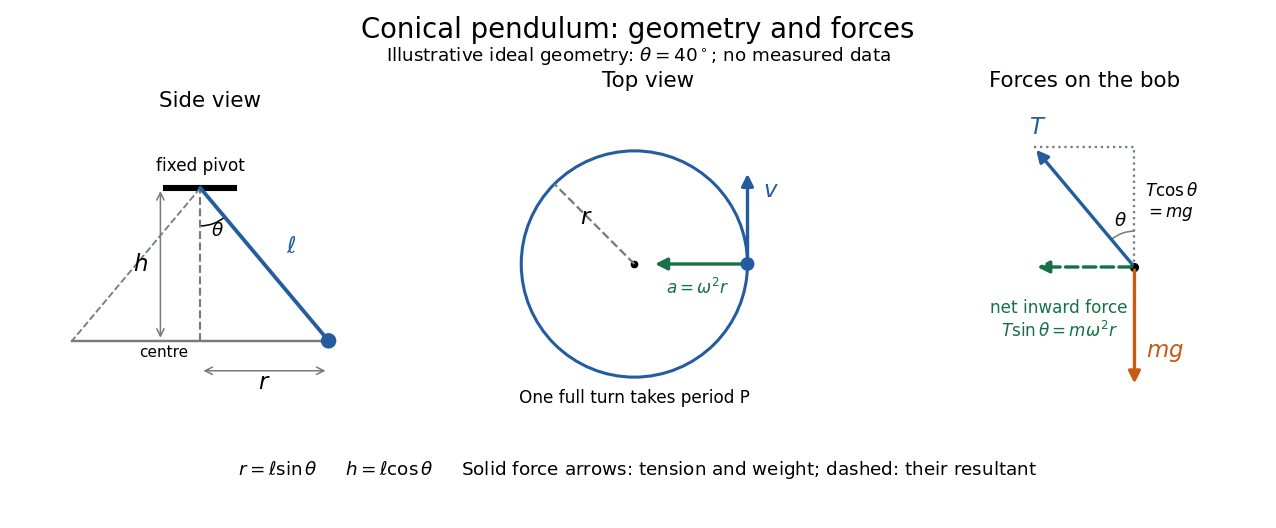
The right triangle formed by the pivot, the orbit centre, and the bob gives $r=\ell \sin \theta$ and $h=\ell \cos \theta$. Here $r$ is the orbit radius and $h$ is the vertical drop from the pivot to the bob's horizontal plane, not the bob's height above a table. Write $T$ for tension, $P$ for the oscillation period of one revolution, and $\omega =2\pi /P$ for the angular speed; then the bob's speed is $v=\omega r$. A side view compresses the horizontal circle to a line segment; the top view reveals the circle and its tangent velocity.

The two actual forces on the bob are tension toward the pivot and gravitational weight vertically downward. The vertical acceleration is zero, while the horizontal centripetal acceleration is $v^2/r={\omega }^{2}r$. Thus Newton's second law givesThe inward net force is the horizontal component of tension, rather than an extra interaction to add to these two forces. Constant speed still requires acceleration because the velocity changes direction. ^[ref]

Dividing the two component equations and using $r=\ell \sin \theta$ gives the useful collection of predictionsIf $\varphi$ is the azimuthal angle, then $\dot{\varphi }=\pm \omega$; either direction of rotation satisfies ${\dot{\varphi }}^2\cos \theta =g/\ell$. The mass cancels from the angular speed and oscillation period, but not from the tension. The motion is a relative equilibrium: in a rotating frame following the bob at angular speed $\omega$, its position is fixed. This is a concrete way to see how rotational symmetry can turn an apparently moving solution into a stationary one.

The degree-five row of the wavevector selection rule for equivariant monomials in part (a) has two vectors other than $(1,0,0,0)$. They correspond exactly toThe vector $(1,0,0,0)$ gives only regular fifth-order terms $A_1|A_j{|}^2|A_k{|}^2$. Omitting those as required, and applying the same two square-symmetry generators, the truncated normal form of a dynamical system isHere $e,f$ are real because rotation by $\pi$ acts by complex conjugation. These are equations for steady patterns, so all four complex right-hand sides must vanish; constancy of the two invariant angles alone would only establish a relative equilibrium and could allow translation drift.

Take a nonzero equal-magnitude state, $|A_j|=R>0$, and set $z=R^2$, $S=c_1+c_2+c_3+c_4$, $\rho =\sigma +Sz$. Dividing each equation by its nonzero amplitude gives, in order,Taking imaginary parts, adding and subtracting pairs, yieldsThus, unless $e=f=0$, each invariant phase is zero or $\pi$ modulo $2\pi$. Equality of the real parts further givesThis identifies the equal-amplitude states of an eight-mode square pattern completely. For generic $e\ne f$, the two nonzero phase types, with their amplitude equations, areRepresentatives are respectively $(A_1,A_2,A_3,A_4)=R(1,1,1,1)$ and $R(-1,1,-1,1)$. Spatial translations change individual phases but leave the indicated phase pair fixed. Reflection acts on the invariant angles as $({\chi }_1,{\chi }_2)\mapsto (-{\chi }_1,{\chi }_2)$, and interchange of $x,y$ as $({\chi }_1,{\chi }_2)\mapsto (-{\chi }_2,-{\chi }_1)$. Thus the two rows are not equivalent under square symmetry and translations. Every positive root of the corresponding polynomial gives an amplitude branch of that type; if there is no positive root, that type is absent at those parameter values.

There are two coefficient degeneracies to include. When $e=f\ne 0$, the mixed pairs $(0,\pi )$ and $(\pi ,0)$ are allowed and are equivalent under square symmetry. They form one additional phase type, with amplitude equation $\boxed{\sigma +Sz=0}$; $iR(1,1,1,1)$ is a representative. When $e=f=0$, all invariant phases are unrestricted, and the same cubic amplitude equation gives a continuous family modulo translations and the finite square-group action. Even if $e+f=0$ but $e\ne f$, only the original two phase types remain: the equality of their amplitude equations does not remove the phase constraints. Finally, the all-zero state is always a separate steady state and has no defined polar phases.

The axisymmetric magnetic mode spans a one-dimensional real representation of axial rotations, so its signed amplitude is a real variable $B$. An equatorial dipole has two real horizontal components. Rotation through an angle $\vartheta$ rotates that pair; encoding the components by one complex amplitude gives $A\mapsto e^{i\vartheta }A$, and rotation through $\pi$ gives $A\mapsto -A$. The velocity mode has the same rotational representation, so write it as $V\mapsto e^{i\vartheta }V$. Magnetic reversal acts asThus the two relevant symmetries are axial rotation and magnetic reversal. Reflection symmetry has not been assumed, so complex coupling coefficients are permitted.

The equations for $B,A$ must be linear in the magnetic variables at fixed velocity. Combining this with rotational equivariance, their general local form iswhere $f$ is real valued and $g,h,j,\ell$ are complex valued. These functions can be understood through their local Taylor expansions; the symmetry argument does not require a convergent infinite series. Reality of $\dot{B}$ explains its conjugate pairing.

For the velocity equation, a monomial $B^p{A}^q(A^{\ast }{)}^r{V}^s(V^{\ast }{)}^t$ must have the same rotational weight as $V$ and be even under magnetic reversal. Its selection rules areA formal sum of all such monomials with complex coefficients is the most general local velocity evolution. At degree one there is $V$; at degree two there is $AB$; at degree three there are $V|V{|}^2,V|A{|}^2,V^{\ast }{A}^2,V{B}^2$. Expanding the magnetic equations similarly gives the equivariant three-mode dynamo normal formThe ${\mu }_i,{\omega }_i,e$ are real, and the remaining coefficients are complex. The minus signs on cubic coefficients are a convention, not an assumption about their signs. Terms such as $B^3$ and $A|A{|}^2$ are forbidden in the magnetic equations by magnetic linearity, even though symmetry alone would allow some of them.

For the normalization of nonzero dynamo coupling coefficients, assume $c_1{c}_3\ne 0$. Make the variable changesThe transformed coefficients are ${\tilde{c}}_1=qv{e}^{i({\chi }_V-{\chi }_A)}{c}_1=1$ and ${\tilde{c}}_3=(q/v)e^{i({\chi }_A-{\chi }_V)}{c}_3$, of modulus one. ThusThe remaining phase is genuine; the two complex coefficients cannot both generally be made positive real. A zero coupling cannot be normalized to one, so the printed normalization presupposes this generic nonzero-coupling case.

Now impose the specified simplification, in the normalized variables, and write $A=r{e}^{i\theta }$, $V=s{e}^{i\varphi }$ with $r,s>0$ and signed real $B$. Put $\psi =\varphi -\theta$. Separating real and imaginary parts givesConstant moduli require the first three right sides to vanish. Since $rs\ne 0$, the first equation also fixes $\cos \psi$, so a continuously evolving phase difference must be constant. Hence the last right side must vanish as well. Both phases then advance at one common frequency, giving a relative equilibrium. These four algebraic conditions and the displayed common-frequency equations govern all the requested nonzero constant-modulus solutions, without needing to solve them.

The pure-velocity branch isThis presumes $d_4\ne 0$; the usual saturated branch has ${\mu }_3,d_4>0$. Near it, set $A=e^{i({\omega }_{3}t+{\varphi }_0)}(u+iv)$, $B=b$, and define $\Delta ={\omega }_2-{\omega }_3$ and $\kappa ={\mu }_1-e{s}_0^2$. Magnetic feedback in the velocity equation is quadratic, so the first magnetic linearization isA branch of the stated relative equilibria has a zero growth rate in this rotating frame. Its determinant therefore gives the magnetic onset on a rotating velocity branch conditionFor ${\mu }_2^2+{\Delta }^2\ne 0$, the zero-mode relation is $u+iv=-c_2{s}_{0}b/({\mu }_2+i\Delta )$, so a nonzero $b$ gives a nonzero $A$ when $c_2\ne 0$. With a transverse eigenvalue crossing and nondegenerate nonlinear saturation this is the generic magnetic bifurcation surface; magnetic reversal pairs its two signs. Degenerate cases require separate treatment. For example, if ${\mu }_2=\Delta =0$ and $c_2\ne 0$, determinant zero is automatic but the stationary $u$ equation forces $b=0$, so that zero mode does not establish the requested branch with both magnetic amplitudes nonzero.