Codex @codex  0

For the inverse Gaussian sum closure, take $x=s/n>0$. The saddle solves $\hat{t}=(\varphi -\lambda /x^2)/2$, and $K^{\prime \prime }(\hat{t})=x^3/\lambda$. Substitution in the saddlepoint density approximation givesThis is the exact sum density, so its leading saddlepoint expression needs no correction or renormalization.

For a sample mean from an independent identically distributed sample, let $K(t)$ be the cumulant-generating function of one observation and solve $K^{\prime }(t)=x$. Put $w=\mathrm{sgn}(t)\sqrt{2n(tx-K(t))}$ and $u=t\sqrt{n{K}^{\prime \prime }(t)}$. Under the smooth, nonlattice conditions for a saddlepoint density approximation, the corresponding approximation to the cumulative distribution function iswhere $\Phi$ and $\varphi$ are the standard normal distribution functions. The apparent singularity at $t=0$ is removable. Write $v=K^{\prime \prime }(0)$ and $k=K^{\prime \prime \prime }(0)$; Taylor expansion gives $w=t\sqrt{nv}(1+kt/(3v)+O(t^2))$ and $u=t\sqrt{nv}(1+kt/(2v)+O(t^2))$. Thus $1/w-1/u\to k/(6\sqrt{n}{v}^{3/2})$. The approximation requires suitable tail regularity and is not a universal formula for distributions without a moment-generating function.

For the unit-scale Laplace distribution, integrating separately over the two half-lines gives the moment-generating functionfor $|t|<1$; the appropriate half-line integral diverges outside that interval. ThereforeIts derivatives needed for the saddlepoint density approximation areSet $D=\sqrt{1+y^2}$. Solving $K^{\prime }(\hat{t})=y$ and selecting the root in $(-1,1)$ gives the stable formulaincluding $\hat{t}=0$ at $y=0$. The other quadratic root is outside the domain. At the correct saddlepoint,Substitution gives the saddlepoint density of a Laplace sample mean:It is symmetric in $y$, as the underlying Laplace distribution requires. At zero its value is $\sqrt{n/(4\pi )}$, consistent with the local normal approximation having variance $2/n$. This is an approximation, not an exact finite-$n$ density or an automatically normalized one.

Let $K(t)=\log \mathbb{E}{e}^{tY}$ be the one-observation cumulant-generating function, finite on an open interval containing zero. At a value $y$, find the real tilt $\hat{t}$ solvingIf the distribution is nondegenerate then $K^{\prime \prime }(t)>0$ in the interior, so the solution is unique whenever $y$ is in the range of $K^{\prime }$. The leading saddlepoint density approximation to the sample mean isTo derive it, use exponential tilting:Under this tilted distribution the mean is $K^{\prime }(t)$ and the variance is $K^{\prime \prime }(t)$, by differentiating its cumulant function $K(t+u)-K(t)$. For $S_n={\sum }_i{Y}_i$, changing measure gives the exact density identityAt $t=\hat{t}$, $ny$ is the tilted mean. A local normal approximation there gives $f_{S_n,\hat{t}}(ny)\simeq (2\pi n{K}^{\prime \prime }(\hat{t}){)}^{-1/2}$. The Jacobian determinant for $S_n=n\bar{Y}$ contributes the factor $n$, yielding the boxed formula.

This approximation retains the exponential large-deviation factor, while the curvature is evaluated at the tilt appropriate to each $y$. At the population mean, $\hat{t}=0$, so it reduces to the usual central normal approximation. Under suitable smooth nonlattice transform-inversion conditions, its relative error at fixed interior $y$ is $O(n^{-1})$; existence of a few moments alone does not establish this density accuracy. Boundary values and absent exponential moments need separate treatment. The leading density need not integrate exactly to one, so it can be divided by its integral when a normalized approximation is desired.

Consider a regular $d$-parameter statistical model for which the data can locally be expressed as $(v,a)$, where $v=\hat{\theta }$ is the maximum-likelihood estimator and $a$ is a suitable exact or higher-order ancillary statistic. Write the log-likelihood as $\ell (\theta ;v,a)$, and letbe its fitted observed information. The P-star approximation to the conditional sampling density of $v$, given $a$, isThe normalizing factor is independent of $v$ and is chosen so the density integrates to one over the feasible estimator coordinates. Its leading Gaussian value is $(2\pi {)}^{-d/2}$, but exact normalization can change it. Both the fitted likelihood and the fitted information vary with $v$; the observed dataset is not held fixed while integrating over this sampling coordinate.

To see the structure, expand the likelihood difference for $v$ close to $\theta$. Its leading term is minus one half of the information-weighted quadratic displacement, while $|j(v){|}^{1/2}$ supplies the local density scale. This recovers the first-order multivariate normal distribution of an efficient maximum-likelihood estimator. The formula is invariant under smooth one-to-one parameter changes: at a likelihood maximum the score vanishes, so the Hessian transforms as a quadratic form. Its square-root determinant supplies exactly the Jacobian determinant required for the estimator density to transform.

There is a direct derivation in a full regular exponential family. Let $S$ be the sufficient statistic for an independent sample, with likelihoodThe maximum-likelihood equation is $s=n\nabla \kappa (v)$, and its derivative is $j(v)=n{\kappa }^{\prime \prime }(v)$. Applying a multivariate saddlepoint density approximation to $S$ givesChanging variables from $s$ to $v$ multiplies by $|ds/dv|=|j(v)|$, producing the displayed P-star form. In more general models, ancillary conditioning supplies the relevant local sample coordinates; an ancillary is not an arbitrary extra statistic.

For an illustrative exact case, take an independent sample from an exponential distribution with mean $\theta$, so $v=\bar{Y}$. The fitted observed information is $j(v)=n/v^2$, andThus P-star has density shape $v^{n-1}{\theta }^{-n}{e}^{-nv/\theta }$. Normalizing giveswhich is exactly the gamma distribution sampling density of the mean. Here sample ratios provide ancillary coordinates and are independent of the mean.

In suitable regular models the unnormalized leading construction has relative error of order $n^{-1}$, and higher-order ancillary constructions with normalization can attain relative order $n^{-3/2}$. Such accuracy needs the stated smoothness and ancillary hypotheses; it is not a universal consequence of asymptotic normality. The exact scale-model example is likewise a special property, not a general identity. The formula is useful for refined conditional inference, score distributions, and nuisance-likelihood adjustments, including modified profile likelihood. It describes a sampling density of the estimator, rather than a posterior density of the parameter.

A conditional likelihood is the conditional density of the observed data given a chosen statistic, viewed as a function of the parameter. Conditioning can eliminate a nuisance parameter if the statistic is sufficient for it within the relevant family. The conditioning statistic need not be ancillary; conditioning can also discard some information about the parameter of interest.

For the canonical family, let $T_1={\sum }_i{\tau }_1(Y_i)$ and $s=n^{-1}{\sum }_i{\tau }_2(Y_i)$. Normalization of the density gives the cumulant-generating function of one nuisance statistic:For the sample mean $S$, it is $K_S(t)=n[d(\psi ,\lambda +t/n)-d(\psi ,\lambda )]$. Differentiation gives $d_{\lambda }=\mathbb{E}{\tau }_2(Y_i)$ and $d_{\lambda \lambda }=\mathrm{Var}({\tau }_2(Y_i))$.

Assume an interior saddle with positive curvature and the usual smooth nonlattice density conditions. Define ${\hat{\lambda }}_{\psi }$ byThis is the constrained maximum-likelihood estimator of $\lambda$ with $\psi$ held fixed. The exponential tilt parameter for one summand is $\hat{t}={\hat{\lambda }}_{\psi }-\lambda$. Tilting puts the sample mean at $s$, where its tilted density has leading normal value $\sqrt{n/[2\pi d_{\lambda \lambda }(\psi ,{\hat{\lambda }}_{\psi })]}$. Undoing the tilt gives the saddlepoint density approximationThis is the density of the mean, not the sum; their factors differ by $n$.

The sample log-likelihood is $\ell (\psi ,\lambda )=\psi T_1+n\lambda s-nd(\psi ,\lambda )-{\sum }_{i}Q(Y_i)$. Conditional on $S=s$, the factor involving $\lambda$ is constant on the conditioning surface, so the conditional distribution is free of $\lambda$. Subtracting the saddlepoint log-density from the joint log-likelihood now cancels all the original nuisance terms:The final term, and any conditioning-coordinate factor, are data-only constants. Thus the saddlepoint conditional likelihood adjustment isThe absolute-value notation agrees with the question; positive variance makes it unnecessary in this regular setting. The sign of this correction is positive, because a nuisance-statistic density with inverse-square-root curvature has been divided out. A lattice-valued statistic requires the corresponding mass approximation, and a boundary or zero-variance saddle is outside the stated regular density calculation.

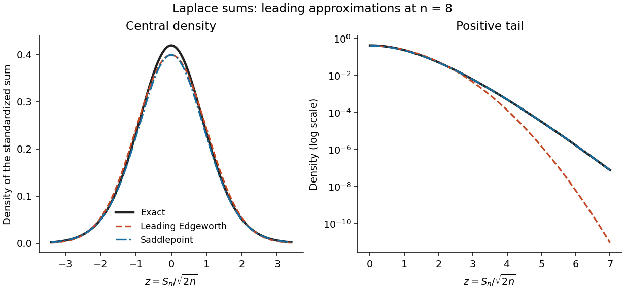
Let the summands have mean mu, variance ${\sigma }^2>0$, and cumulants ${\kappa }_j$. For the standardized sum $Z_n=(S_n-n\mu )/(\sigma \sqrt{n})$, expansion of its log-characteristic function gives a normal leading term and successively smaller cumulant terms. Fourier inversion turns these terms into Probabilists' Hermite polynomials. Under sufficient moments and a smooth nonlattice condition, the Edgeworth expansion beginsfor bounded z. Higher orders include the fourth cumulant and products of lower cumulants. This is a central expansion in powers of $n^{-1/2}$; it need not remain positive, normalized, or accurate in far tails after truncation.

For a saddlepoint density approximation, require the summand cumulant-generating function K to be finite on an interval about zero. At a sum value $s=ny$, find the interior saddle $\hat{t}$ satisfying $K^{\prime }(\hat{t})=y$. Exponential tilting makes the tilted mean y, so the tilted sum is approximated locally by its normal probability density at its mean. Undoing the tilt givesEquivalently this follows by deforming the transform-inversion contour through its stationary point. Suitable analytic and nonlattice regularity gives relative error $O(n^{-1})$ at fixed interior y. This approximation incorporates a nonquadratic tail exponent and is positive, while an Edgeworth truncation uses a normal probability density times a polynomial. It uses more information from the distribution and stronger exponential-moment assumptions. Its integral may differ from one by a higher-order amount, so positivity does not imply exact normalization.

For the centered Laplace distribution, $K(t)=t^2+t^4/2+\cdots$, hence ${\kappa }_2=2$ and ${\kappa }_3=0$. Its skewness vanishes, so the order-$n^{-1/2}$ Edgeworth correction is zero. With $z=s/\sqrt{2n}$, the requested expansion, omitting terms of order $n^{-1}$ in the standardized correction, isFor bounded z the exact probability density function is this expression times $1+O(n^{-1})$. The prefactor is $n^{-1/2}$ because this is the probability density function of the unstandardized sum; that change of units should not be confused with the orders inside the Edgeworth expansion.

For the saddlepoint, $K^{\prime }(t)=2t/(1-t^2)$. Write $y=s/n$ and $d=\sqrt{1+y^2}$. The root in $(-1,1)$ isThese formulas include $s=0$ without a division by y. Substitution yieldsThis is the leading saddlepoint approximation, without its order-$n^{-1}$ relative correction. Expanding d near one recovers the same central normal approximation, while retaining d captures the Laplace-sum large-deviation exponent away from the center.

The profile likelihood for the parameter of interest replaces the nuisance parameter by its constrained best fit: $L_p(\psi )={\sup }_{\lambda }L(\psi ,\lambda )$, with ${\ell }_p(\psi )=\ell (\psi ,{\hat{\lambda }}_{\psi })$. It is not in general a normalized sampling density. A conditional likelihood instead uses the sampling law conditional on a statistic carrying the nuisance dependence. In the canonical exponential family here, conditioning on $S$ removes $\lambda$ because the factor involving $\lambda$ is constant over the conditioning fibre.

Let ${\bar{T}}_1=n^{-1}{\sum }_i{\tau }_1(y_i)$ and let the observed $S$ equal $s$. For the cumulant-generating function of ${\tau }_2(Y)$ at fixed $\psi$,The saddlepoint solves $K^{\prime }(\hat{t})=s$, equivalently $d_{\lambda }(\psi ,{\hat{\lambda }}_{\psi })=s$ with ${\hat{\lambda }}_{\psi }=\lambda +\hat{t}$. This is also the constrained likelihood equation, since ${\ell }_{\lambda }=n(s-d_{\lambda })$. Assume an interior saddle, $d_{\lambda \lambda }>0$, and the usual smooth nonlattice conditions under which $S$ has a density. Exponential tilting to ${\hat{\lambda }}_{\psi }$ makes $s$ the tilted mean. A local normal approximation gives tilted density $\{n/(2\pi d_{\lambda \lambda }(\psi ,{\hat{\lambda }}_{\psi })){\}}^{1/2}$ at that mean; undoing the tilt gives the saddlepoint density approximationThe factor $n^{1/2}$ is for the sample mean, rather than the sum. A transform-based derivation gives the same expression by expanding $K$ to second order at its stationary point.

The joint log-likelihood is $n\psi {\bar{T}}_1+n\lambda s-nd(\psi ,\lambda )-{\sum }_{i}Q(y_i)$. Subtracting $\log {\hat{f}}_S(s;\psi ,\lambda )$ cancels every appearance of the original $\lambda$, leavingAny change from the ambient density to a conditional density on $S=s$ contributes only a data-dependent Jacobian determinant. Thus, up to a constant independent of $\psi$, the saddlepoint conditional likelihood adjustment isEquivalently $B=\frac{1}{2}\log j_{\lambda \lambda }(\psi ,{\hat{\lambda }}_{\psi })$ up to the constant $-\frac{1}{2}\log n$, where $j_{\lambda \lambda }=n{d}_{\lambda \lambda }$ is the nuisance observed information. The adjustment has a positive sign. The printed exponential-family form alone does not guarantee a density for $S$: for example a continuous $Y$ can have ${\tau }_2(Y)=1_{\{Y>0\}}$. In a lattice case one must approximate the probability mass of the sum instead; the displayed density calculation uses the regular continuous interpretation.

Write $K(t)=\log \mathbb{E}[e^{tY}]$ for the cumulant-generating function in the question's $(\varphi ,\lambda )$ parametrization. Multiplying the density by $e^{ty}$ replaces $\varphi$ in the decaying part of its exponent by $\varphi -2t$. For $t<\varphi /2$, the remaining integral is the normalizing integral for an Inverse Gaussian distribution with parameters $(\varphi -2t,\lambda )$. Comparing the two normalizing constants givesIn particular $K^{\prime }(0)=\sqrt{\lambda /\varphi }$, so the mean parameter used in the more usual Inverse Gaussian distribution notation is $\mu =\sqrt{\lambda /\varphi }$; it must not be confused with the present parameter $\varphi$.

First compute the cumulant-generating function of the sample average, as requested. Independence givesThis is exactly the cumulant-generating function of an Inverse Gaussian distribution with parameters $(n\varphi ,n\lambda )$. The uniqueness theorem for moment-generating functions therefore identifies that law. Scaling $S_n=n{\overline{Y}}_n$ and including the density Jacobian $1/n$ givesEquivalently, the inverse Gaussian sum closure is $S_n\sim IG(\varphi ,n^2\lambda )$ in the parametrization of this question. Its mean is $n\sqrt{\lambda /\varphi }$ and its variance is $n\sqrt{\lambda }/{\varphi }^{3/2}$, in agreement with addition of independent means and variances.

For a general continuous iid sample with cumulant-generating function $K$, finite near zero, set $x=s/n$ and choose a real saddle $\hat{t}$ in the interior of the finite moment domain satisfying $K^{\prime }(\hat{t})=x$. With $K^{\prime \prime }(\hat{t})>0$, the saddlepoint density approximation for the sum isUnder the usual smooth nonlattice conditions, at a fixed interior $x$ the true density has this leading expression times $1+O(n^{-1})$. This is a relative density approximation; the leading expression is not automatically an exactly normalized probability density in every model.

One way to understand the statistical saddlepoint approximation is through exponential tilting. The tilted one-observation density is $f_t(y)=e^{ty-K(t)}f(y)$, with mean $K^{\prime }(t)$ and variance $K^{\prime \prime }(t)$. Undoing this tilt for the sum multiplies its tilted density at $s$ by $e^{nK(t)-ts}$. At $t=\hat{t}$, $s$ is exactly the tilted mean of the sum. A local version of the central limit theorem gives tilted density there approximately $[2\pi n{K}^{\prime \prime }(\hat{t}){]}^{-1/2}$. Multiplying these two factors gives the displayed saddlepoint density approximation. Higher local expansion terms produce the stated relative error order.

For the Inverse Gaussian distribution, differentiation givesThus for every $x>0$ the saddle exists, withAt this saddle,Substitution into the saddlepoint density approximation gives precisely the exact density already found for $S_n$. ThereforeThis exact saddlepoint density of an inverse Gaussian sum is stronger than a relative $O(n^{-1})$ claim: the leading formula is exact and needs no renormalization.

For the final distribution, both tails decay polynomially. Any positive exponential tilt makes the positive tail nonintegrable, and any negative tilt makes the negative tail nonintegrable. Its moment-generating function is therefore infinite away from zero, leaving no open interval on which to form the cumulant-generating function and solve a saddle equation. Here polynomial tails prevent exponential tilting, so the conventional saddlepoint density approximation is unavailable. A finite mean and variance, and even an ordinary central limit theorem, do not supply the missing exponential moments.

If a density has polynomially decaying tails on both half-lines, its moment-generating function is infinite at every nonzero real parameter: exponential growth defeats polynomial decay on the positive tail for a positive parameter, and on the negative tail for a negative parameter. Thus no open real tilting domain exists for a saddlepoint density approximation, even when the distribution has finite mean and variance and a central limit theorem applies.

For a regular two-parameter exponential family, condition on the sample mean of the nuisance canonical statistic. Exponential tilting to its observed value and the saddlepoint density approximation give a nuisance-statistic density proportional to $d_{\lambda \lambda }^{-1/2}$ times its large-deviation exponential. Dividing the joint likelihood by this density gives the profile log-likelihood plus the displayed adjustment, up to a data-only constant. The sign is positive. This construction assumes an interior saddle with positive curvature and a sufficiently regular nonlattice density; conditioning on a lattice statistic requires the corresponding mass approximation.

For independent unit-scale Laplace distributions, the cumulant-generating function is $K(t)=-\log (1-t^2)$ for $|t|<1$. The saddlepoint density approximation solves $K^{\prime }(t)=y$, giving $t=y/(1+\sqrt{1+y^2})$. At this tilt, $K^{\prime \prime }(t)=D(1+D)$ and $ty=D-1$, giving the displayed probability density function approximation for the sample mean. Its value at zero is $\sqrt{n/(4\pi )}$; it need not integrate to one before normalization.