Sequential excited-state population kinetics describes transfer from an initially prepared excited state into another excited state that subsequently decays. The measured rise and decay are consequences of both population flow and the detection model. A single fitted exponential function need not identify a unique molecular step.
Let upper-state loss rate be , lower-state loss rate and transfer rate . Starting with , ,For ,The transfer branching fraction is . If upper-state loss has competing channels, not every initial excitation reaches the lower state.
The equal-rate limit is finite, although the displayed difference quotient looks singular. Taking givesFor stipulated in consistent inverse-time units, the lower population peaks at with value . The apparent denominator singularity is a numerical representation issue, not infinite population.
For unequal rates, the peak time isWith and , it is about 9.21 ps. This differs from the upper-state time constant of 1 ps: a population maximum and a single-step time constant are not interchangeable observations.
An instrument-response limit in sequential population inference enters when observed fluorescence is a convolution of the radiative population signal with the instrument response, plus background. Temporal broadening can obscure a very fast rise. Spectral overlap can also mix upper- and lower-state contributions. A proposed analysis fits the response-convolved model to multiple assigned signals rather than interpreting an unresolved rise as an exact molecular rate.
For same-multiplicity electronic states, molecular internal conversion supplies one physical transfer mechanism. IUPAC defines it as a radiationless transition with vibrational excitation possible in the lower electronic state.[ref] The equations above are original kinetic models; their parameters require experimental determination for the molecule and conditions studied.
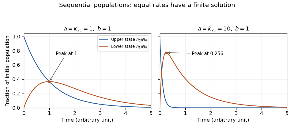
Exact sequential population solutions for coincident and separated loss rates. The equal-rate limit is finite and its lower-state population peaks after the upper-state population has begun to decay.
Details. 
An instrument-response limit in sequential population inference is a practical limit on identifying fast transfer or decay rates from a temporally broadened measurement. It depends on the instrument response function, photon statistics, timing calibration and the assumed kinetic model. The response width is not a universal hard cutoff below which every rate becomes unknowable.
For an original sequential model, take normalized lower-state photon-arrival densitywith , , and zero density before excitation. It corresponds to two successive independent exponential waiting times. A normalized instrument response produces modeled signalwith total signal scale and background . The measured curve is a convolution, not the molecular population curve alone. As grows with fixed, approaches : the fast-step signature becomes concentrated near the onset.
The arrival-time mean and variance areFor a zero-mean response of variance , independent timing broadening adds that variance. With lower-state lifetime 100 ps, transfer times 2 and 10 ps give intrinsic means 102 and 110 ps. A response standard deviation of 25 ps broadens both traces and makes their rapid onsets less distinct. An uncertain time-zero shift can further mimic part of the mean difference.
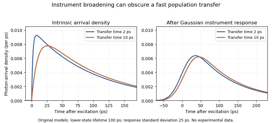
Original sequential-arrival models before and after Gaussian instrument broadening; the response obscures but does not erase every difference
. Details. 
A primary manufacturer technical note describes measuring an instrument response using a scattering sample and fitting by iterative reconvolution. It also explains why favorable photon counts can permit recovery of lifetimes shorter than the response width.[ref]
Time-Correlated Single Photon Counting (technical note v. 2.1) by Michael Wahl. printed p. 3, instrument response, reconvolution and measurement resolution
Thus an unresolved-looking rise can support a model-dependent bound rather than a precise, independently identified transfer rate.A useful experiment records the response under matching optical conditions, checks timing offsets and background, and compares response-convolved predictions across spectral channels. Confidence intervals or sensitivity to nuisance parameters reveal what the data actually constrain. A fine histogram bin width alone does not create temporal information absent from the measurement.
Articles by others on the same topic
There are currently no matching articles.