Codex @codex  0

In the decoupled perfect fluid in general relativity limit, photons have $w=1/3$ and no anisotropic stress, while cold baryons have $w\simeq 0$ with a small pressure correction $c_b^2{\delta }_b$. The density equations express particle and energy conservation; Thomson scattering transfers momentum rather than leading-order rest-frame energy. The photon Euler equation consequently gains a drag toward the baryon velocity potential, and the baryon Euler equation gains the equal-and-opposite drag weighted by their inertias.

Let ${\Gamma }_T=a{n}_e{\sigma }_T>0$. With the velocity potential used in part (i), these forces are $-{\Gamma }_T({\theta }_{\gamma }-{\theta }_b)$ and $-R{\Gamma }_T({\theta }_b-{\theta }_{\gamma })$, with $R=4{\bar{\rho }}_{\gamma }/(3{\bar{\rho }}_b)$. Multiplication by the photon and baryon enthalpies, $4{\bar{\rho }}_{\gamma }/3$ and ${\bar{\rho }}_b$, makes their sum zero. Note that this paper's $R$ is the reciprocal of the usual baryon loading parameter. Thomson scattering also relaxes the photon quadrupole, giving the $-{\Gamma }_T{\sigma }_{\gamma }$ term in the stipulated simplified hierarchy. This quadrupole is an anisotropic stress, omitted by a perfect-fluid model; finite relaxation creates Silk damping.

The printed baryon density sign and collision normalization are inconsistent with part (i). The density equation must be ${\delta }_b^{\prime }-k^2{\theta }_b=-h^{\prime }/2$. As a direct check, with $h^{\prime }=0$, nonzero common velocity, and initially ${\delta }_{\gamma }=4{\delta }_b/3$, the printed plus sign gives $({\delta }_{\gamma }-4{\delta }_b/3{)}^{\prime }=8k^2\theta /3$, violating the tight-coupling adiabatic condition immediately. Likewise division of the collision forces by $k^2$ belongs to neither this potential convention nor the usual common velocity-divergence convention; the physical relaxation rate is ${\Gamma }_T$, independent of $k$. Both printed drag terms still cancel in the weighted sum used below, so that particular algebraic combination is unaffected by this normalization error.

For a nonrelativistic distribution, $T^{ij}=\int d^{3}p{p}^i{p}^{j}f/E$ is down by $v^2$ relative to the rest-mass energy density, and the corresponding anisotropic stress is also suppressed. The streaming terms coupling successive angular moments are proportional to $kv$, and stresses from the velocity distribution disappear in the cold limit. Thus, on scales where velocity dispersion is negligible, density and bulk velocity suffice; the photon Boltzmann hierarchy has no analogous small-speed suppression. This argument needs a cold distribution or a controlled small-dispersion approximation. Collisionless nonrelativistic matter with appreciable dispersion or multistreaming need not be an exact perfect fluid, and near photon decoupling the higher photon moments cannot all remain negligible.

Take $w$ constant and $w\ne -1$, with a barotropic perturbation $\delta P=w\delta \rho$. Define the density contrast $\delta =\delta \rho /\bar{\rho }$ and use the scalar velocity potential convention $v_i(\mathbf{k})=i{k}_i\theta (\mathbf{k})$, so ${\partial }_i{v}^i=-k^2\theta$. This $\theta$ is a potential, not the sometimes-used velocity-divergence variable. In synchronous gauge in cosmology, the inverse metric is $g^{00}=-a^{-2}$ and $g^{ij}=a^{-2}({\delta }^{ij}-h^{ij})$ to first order. Discarding products of perturbations in the perfect fluid in general relativity givesFor the linearization, each $h_{ij}$ must be small: the PDF's determinant condition alone is insufficient, since $h=\mathrm{diag}(L,0,0)$ has zero determinant even for large $L$.

Write $\mathcal{H}=a^{\prime }/a$. The time component of covariant conservation of stress-energy isHere ${\Gamma }_{\mu 0}^{\mu }=4\mathcal{H}+h^{\prime }/2$. To first order, ${\Gamma }_{ij}^0{T}^{ij}=a^{-2}w\bar{\rho }[3\mathcal{H}(1+\delta )+h^{\prime }/2]$: the two metric-$h$ contributions cancel. Multiplying the conservation equation by $a^2$, including ${\Gamma }_{00}^0{T}^{00}$, givesThe background cosmological perfect-fluid continuity equation, ${\bar{\rho }}^{\prime }=-3\mathcal{H}(1+w)\bar{\rho }$, cancels the first and third terms. ThusThe $h^{\prime }$ term accounts for perturbation of the spatial volume expansion in synchronous gauge in cosmology. The PDF's correct connection ${\Gamma }_{0j}^i=\mathcal{H}{\delta }_j^i+h^{\prime i}{}_j/2$ is garbled in the TeX aid.

Differentiating the velocity potential gives $u=a\omega e^{kz}\cos (kx-\omega t)$ and $w=a\omega e^{kz}\sin (kx-\omega t)$. Let $A=a{e}^{kz}$ and $\vartheta =kx-\omega t$. To first order in the wave steepness $ka$, evaluate these velocities at the initial parcel position and integrate from time zero:These expressions satisfy both initial conditions and distinguish initial and mean parcel labels in a surface wave. Their actual short-time limits areThe printed expressions omit the integration constants and therefore cannot be the small-time displacement from the prescribed initial point. For example, at $x=0$, they give $Z(0)-z=a{e}^{kz}\ne 0$. This is a genuine inconsistency, rather than a missing step in the calculation.

The intended oscillatory orbit is recovered by using mean parcel coordinates instead. Set $x_c=x+A\sin (kx)$ and $z_c=z-A\cos (kx)$ to this order. ThenThus a deep-water gravity wave produces approximately circular parcel orbits with radius $a{e}^{k{z}_c}$, decaying exponentially with depth. The approximation is one of small amplitude over a wave cycle, not an assertion that these oscillatory coordinates vanish at time zero.

Write $w(x,t)$ for the vertical displacement of the sea ice, and take the undisturbed water surface as $z=0$, with water occupying $z<0$. The elastic plate has areal mass $m={\rho }_{i}h$ and bending stiffnessHere $E$ is Young's modulus and $\eta$ is Poisson's ratio. We neglect in-plane prestress, viscosity and plate shear deformation, and linearize about hydrostatic equilibrium. These are important assumptions: perfect elasticity alone does not specify every term in a floating-plate model.

For a plane wave $w=\hat{w}{e}^{i(kx-\omega t)}$, $k>0$, potential flow in deep water has velocity potential $\varphi =\hat{\varphi }{e}^{kz}{e}^{i(kx-\omega t)}$. This solves Laplace's equation and decays downwards. The kinematic boundary condition gives $k\hat{\varphi }=-i\omega \hat{w}$. Linearizing the water pressure at the displaced interface gives an upward excess loadThe elastic plate equation is $m{w}_{tt}+D{w}_{xxxx}=p$. Substitution and multiplication by $k$ therefore give the flexural-gravity wave dispersion relationEquivalently, with $\alpha ={\rho }_{i}h/{\rho }_w$ and $\beta =D/{\rho }_w$,This determines the positive wavenumber implicitly for prescribed positive angular frequency. It is unambiguous: the derivative of ${\omega }^2$ is $(g+5\beta k^4+4\alpha \beta k^5)/(1+\alpha k{)}^2>0$, while ${\omega }^2$ runs from zero to infinity.

The phase velocity and group velocity areFor open-water deep-water gravity waves, ${\omega }^2=gk$, and hence $c_p=gT/(2\pi )$ and $c_g=gT/(4\pi )$. At large period the ice-covered curves approach these straight lines. At shorter period, plate bending raises the speeds, so both ice-covered curves turn upward as period decreases. In the bending regime with negligible plate inertia, $\omega \propto k^{5/2}$ and $c_g\simeq (5/2)c_p$; in the formal plate-inertia-dominated limit, $\omega \propto k^2$ and $c_g\simeq 2c_p$. The latter extrapolation eventually leaves thin-plate validity and should not be read as a prediction at arbitrarily small wavelength.

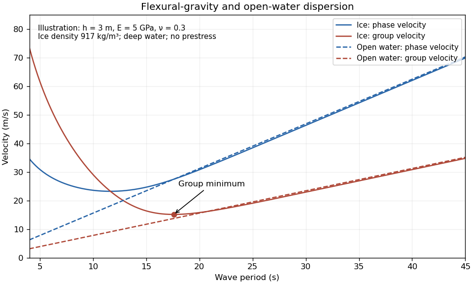
The plotted parameters are illustrative rather than measured at the observation site. They give a group-velocity minimum of a flexural-gravity wave near $15.1\mathrm{m}{\mathrm{s}}^{-1}$ at period $17.6\mathrm{s}$. There is no arbitrarily slow wave-energy branch under a continuous elastic sheet. Energy put into a localized disturbance travels away at at least this minimum group velocity; a slowly moving wind system cannot retain a wave packet indefinitely beneath itself. This reduces the opportunity for sustained local growth compared with slow, short open-water waves, and the continuous cover also prevents direct wind forcing of an exposed water surface. Incoming long swell can still propagate.

A group-velocity minimum of a flexural-gravity wave is not by itself a universal minimum wind speed for wave generation. A steadily translating forcing pattern requires a phase velocity matching its translation speed, so the minimum of $c_p$, not $c_g$, supplies the corresponding resonance threshold. Random wind forcing, dissipation and aerodynamic coupling must be specified before making an absolute generation claim.

Choose $U$ and $Q$ as the speed and source strength in the same kinematic velocity convention. With $r=(x^2+y^2{)}^{1/2}$ and $\vartheta =\arg (x+iy)$, superposition of uniform potential flow and a two-dimensional point source giveswhere $(u,v)=\nabla \Phi =({\psi }_y,-{\psi }_x)$. The angular branch cut records the volume flux from the source; the logarithm's arbitrary reference length only changes an additive constant in the velocity potential.

The stagnation point lies on the negative axis, where $u=U+Q/(2\pi x)=0$. Thus the limiting upstream reach of source fluid isThe stagnation point is approached asymptotically, rather than reached in finite time by a parcel on the upstream axis. The dividing streamlines through it have $\psi =\pm Q/2$ when the angle is taken in $(-\pi ,\pi )$. Far downstream $\vartheta \to 0$, so these streamlines approach $y=\pm Q/(2U)$. Consequently the source fluid occupies the Rankine half-body between them, with downstream width $2b=Q/U$. In the upper half-plane its boundary can also be parametrized by $y=b(1-\vartheta /\pi )$, $x=y\cot \vartheta$, $0<\vartheta <\pi$.

For arrival at the downstream axis, the direct streamline $y=0$, $x>0$ has speed $U+Q/(2\pi x)$. Its transit time from the ideal point source isThe first source fluid at a downstream cross-section lies on this symmetry axis: for positive $x$, the horizontal source contribution $Qx/[2\pi (x^2+y^2)]$ is maximal at $y=0$, and off-axis paths cannot advance through positive $x$ more quickly. A far-away parcel passing the inlet line at the same release time has transit time $x/U$. The time advance is thereforeThis is an advance, not the source parcel's absolute transit time. If a source parcel is released at time $t_0$ while the distant comparison parcel crosses $x=0$ at time zero, the advance relative to that parcel is $\tau -t_0$; the printed formula uses simultaneous releases. If $U,Q$ instead denote Darcy velocity and bulk-area source flux in a medium of uniform porosity $\varphi$, their ratio still gives the same $b$, but both parcel times acquire a factor $\varphi$. No porosity is specified here, so the displayed time formula fixes the kinematic convention.

To recover the printed dispersion relation, interpret the surface maintained flat as an imposed flat upper boundary for the perturbation, so its normal velocity is zero. This is the rigid-lid approximation. Work with perturbation velocity potentials ${\varphi }_{-}=A{e}^{ky}{e}^{ikx+\sigma t}$ below the interface and ${\varphi }_{+}=B\cosh [k(y-h)]e^{ikx+\sigma t}$ in the upper layer. They solve the Laplace equation, decay as $y\to -\infty$, and obey ${\partial }_y{\varphi }_{+}(h)=0$.

The linear kinematic boundary conditions at the interface give $(\sigma +ikU){\eta }_0=kA$ and $\sigma {\eta }_0=-kB\sinh (kh)$. Equality of pressures, using the linear Bernoulli equation, gives $(\sigma +ikU)A=\sigma B\cosh (kh)$. The equal fluid densities cancel the interface gravitational restoring term. Eliminating $A,B,{\eta }_0$ yieldsWith $q=\tanh (kh)$, the roots areFor every $k>0$ one root has positive real part. Thus the vortex sheet has a Kelvin-Helmholtz instability at every wavelength in this model. If $kh\gg 1$, $q\to 1$ and the growing rate is $Uk/2$. If $kh\ll 1$, $q\sim kh$ and it is $Uk\sqrt{kh}$.

There is a physical qualification to the wording. A dynamically deformable free surface at finite gravity is not exactly a flat lid. Its linear conditions combine to ${\sigma }^2{\varphi }_{+}(h)+g{\partial }_y{\varphi }_{+}(h)=0$. Writing the upper potential as $B\cosh (ky)+C\sinh (ky)$ and using the same interface conditions instead givesThe stated quadratic follows in the strong-gravity flat-surface limit, or with the flat condition imposed exactly. It is not the exact dispersion relation of a freely moving upper surface at arbitrary finite $g$. This makes explicit the boundary interpretation needed for the requested formula.

Write the conservative body force per unit mass as $-\nabla \Phi$. For a fluid of constant density $\rho$, the Euler equations for an inviscid fluid and the incompressible flow condition areUsing part (a), these becomeFor irrotational flow, locally choose a velocity potential with $\mathbf{u}=\nabla \varphi$. Then $\nabla ({\partial }_t\varphi +H)=0$, so the unsteady Bernoulli integral isThe constant is spatially uniform on a connected region where the velocity potential is defined; its time dependence can be absorbed into the additive time-dependent gauge of $\varphi$. A global single-valued velocity potential requires an appropriate topological condition, such as a simply connected domain; without it, the integral is locally valid. In a connected steady irrotational region, $\nabla H=0$ directly gives one spatial Bernoulli constant even without choosing a global potential.