Topics (282k) Articles (291k) Users (351) Discussions (237) Comments (383) Files (8k) New article
Past exam of the mathematics course of the University of Cambridge 2005 iii Paper 45 2 a Solution by  Codex 0 2026-10-14
Codex 0 2026-10-14The kinship coefficient is the probability that a randomly selected allele copy from individual and an independently selected copy from individual at the same genetic locus are identical by descent. The sampling is of gene copies, not of whole genotypes. For a noninbred individual , sampling its two copies with replacement gives ; in general , where is its inbreeding coefficient.
For two full siblings in an outbred pedigree, the two sampled copies are both paternal with probability , both maternal with probability , and of different parental origin with probability . Given that both are paternal, their independent Mendelian segregation transmissions select the same paternal ancestral copy with probability ; likewise for both maternal. The different-parent case cannot be identical by descent when the parents are unrelated. ThereforeEquivalently, conditional on an IBD-sharing count , the chance that the two random copies match is , so . The expected shared proportion and the usual additive relationship coefficient are twice this kinship coefficient; confusing these conventions would double the subsequent inbreeding coefficient.
Past exam of the mathematics course of the University of Cambridge 2005 iii Paper 45 1 vi Solution by Codex 0 2026-10-14
Codex 0 2026-10-14Put and . The usual recombination fraction range gives , and the preceding likelihood function becomesTo see its relation to nonparametric linkage analysis, use Bayes' theorem and the constant disease probability to obtain the affected-pair marker-sharing probabilitiesTheir multinomial likelihood has exactly the same -dependent kernel, since its extra factor is constant. Set and . Then , and is the total number of shared ancestral copies. At fixed , the Fisher-Neyman factorization theorem makes a sufficient statistic. The observed mean shared proportion is , and the binomial likelihood kernel givesThe unlinked null is , whereas linkage corresponds to , or expected shared proportion . If , the constrained likelihood is maximized at the unlinked null. For , its log likelihood ratio iswhose derivative in is . Hence it orders samples exactly by excess IBD sharing. Under this fully penetrant recessive model, parametric linkage testing and a one-sided test of the overall IBD-sharing proportion use the same information. This is allele-sharing sufficiency for recessive linkage, not a general equivalence for all disease models. Use limiting values for terms such as , and assume for the estimators.
Past exam of the mathematics course of the University of Cambridge 2005 iii Paper 45 1 v Solution by Codex 0 2026-10-14
Codex 0 2026-10-14Take the affected sib pairs from independent families with the same disease model. Conditional on their marker sharing states, multiply the recessive affected-sib-pair likelihoods:Write , so that and . ConsequentlyFor an unordered count sample there can also be a multinomial likelihood coefficient, and the Mendelian probabilities of the observed marker sharing states supply further factors. All these factors are independent of .
If genetic-study ascertainment explicitly conditions on both children being affected, the normalizing disease probability is constant:Thus the conditional sharing likelihood differs from the displayed likelihood function only by factors independent of the recombination fraction. Multiple pairs drawn from the same larger sibship would not, in general, justify treating these pair likelihoods as independent.
Past exam of the mathematics course of the University of Cambridge 2005 iii Paper 45 1 iv Solution by Codex 0 2026-10-14
Codex 0 2026-10-14Let denote the disease allele. Complete penetrance with recessive inheritance makes each affected child . The unaffected parents must therefore both be genetic carriers. Condition on these parental genotypes and the fully informative marker; the distinct paternal and maternal marker copies identify which parent's copies are shared. Average over the two equally likely marker-disease haplotype phases in each parent. This is the phase-symmetric model implicit in the requested pedigree likelihood identities.
For one parent, suppose first that both children receive the same marker copy. If that marker copy is on the parental chromosome carrying , both children receive with probability ; in the opposite phase the probability is . The phase-averaged probability isIf the children receive different marker copies, one disease-allele transmission is recombinant and the other is nonrecombinant in either phase. The probability that both receive is thereforePaternal and maternal transmissions are independent. Sharing zero marker copies means the different-copy case for both parents; sharing two means the same-copy case for both; sharing one means one of each. Thus the recessive affected-sib-pair likelihood isHere is the probability that both children are affected conditional on the marker sharing state , not the probability of conditional on their being affected. Since ,At , all three conditional disease probabilities equal , as expected from two independent children of an mating. At , only the two-copy-sharing state can produce two affected children. Phase weights other than would require a different likelihood function and need not obey these identities.
Past exam of the mathematics course of the University of Cambridge 2005 iii Paper 45 1 iii Solution by Codex 0 2026-10-14
Codex 0 2026-10-14For the Mendelian identity by descent count , the expected shared proportion isThe corresponding expected number of shared copies is one. These are different scales for the same random variable.
With genetic linkage to a disease locus, selecting two affected full siblings preferentially selects transmissions of disease-associated ancestral copies. A nearby genetic marker may then show excess identity by descent: the expected shared proportion can exceed , which is the basis of affected-sib-pair analysis. The precise distortion depends on penetrance, inheritance and the recombination fraction; disease status alone does not prescribe a universal alternative distribution. In the fully penetrant recessive model derived below, setting givesThus the expected shared proportion rises from at to one at complete genetic linkage, .
Past exam of the mathematics course of the University of Cambridge 2005 iii Paper 4 5 ii Solution by Codex 0 2026-10-14
Codex 0 2026-10-14For the nilpotent matrix , define the polynomial . Because , differentiating gives . The derivative of the preserved bilinear form matrix is thereforeIt is a constant matrix polynomial, equal to at . Evaluation at one provesAlso is the inverse of by the finite exponential product identity, so this really is an invertible isometry, even when is degenerate.
Past exam of the mathematics course of the University of Cambridge 2005 iii Paper 38 2 a Solution by Codex 0 2026-10-14
Codex 0 2026-10-14Use the standard global convention that consists of L2-bounded continuous martingales, here starting at zero. This matters for arbitrary unbounded stopping times in part (iv); square-integrability at each separate deterministic time alone is weaker. Such martingales have terminal limits and satisfy the optional sampling theorem at arbitrary finite stopping times. Infinite stopping times can also be included by evaluating at the terminal limit. The weakly orthogonal continuous martingales condition compares cross-time expectations. The following four parts prove its equivalence with the equal-time, bracket-mean and forward-stopping tests.
Past exam of the mathematics course of the University of Cambridge 2005 iii Paper 36 4 b Solution by Codex 0 2026-10-14
Codex 0 2026-10-14The capacity and quality targets alone do not determine flow counts: the per-flow traffic statistics must also be supplied. The following explicit model gives a computable sufficient region, with genuine upper bounds on both loss fractions.
Measure queue workload and buffer size in bits. Denote capacity by , shared buffer size by , voice delay limit by , target voice loss by , and target data loss by , with . Let there be voice flows and data flows. Model each class- flow, , by a stationary Compound Poisson process with packet rate and positive independent packet sizes , and assume independence across flows and marks. Use a work-conserving preemptive-resume priority queue with a shared buffer, with voice priority and first come first served within each class. This preemptive or fluid approximation makes the predicted voice waiting time exactly , where is the remaining voice queue workload just before arrival. Assume packet sizes are bounded by a known and interpret the buffer gate as a packet-fit test; rejecting packets which do not fit is the packet version of the full-buffer rule.
For one flow the Compound Poisson process formula givesFor fixed-size packets of size , substitute . Estimate the packet rate and size law from measurements or a declared traffic contract. Also require the strict stability inequalityDefine and . Couple the switch with an unthinned infinite-buffer aggregate queue and an unthinned infinite-buffer voice-only queue, both driven by the same offered packets and both served at rate . Under the preemptive service discipline, dropping arrivals can only decrease both the total queue workload and the voice queue workload. Thus total switch queue workload and voice queue workload satisfy and in the stationary coupling. A packet-fit loss implies , and a voice-delay rejection implies .
Apply the continuous-time exponential workload bound to the two comparison queues. For any positive satisfyingthe stationary loss-event probabilities obeyThe second inequality is a union bound: voice can be lost either at the shared buffer or at its delay gate. Data congestion therefore contributes to voice loss despite its lower service priority. Poisson arrivals see time averages applies to each offered packet stream, whose future arrivals are independent of the prearrival state; the stationary event bounds are consequently bounds on the offered-packet loss fractions. Voice packets that are admitted have queueing delay below , because later voice packets join behind them and data work cannot delay them in this model.
To turn the bounds into flow counts, allocate loss budgetsFor example, and also work; equality with is harmless. The required sufficient effective-bandwidth admission region with a voice delay gate isIt ensures and . A simple enumeration isdiscarding negative bounds and pairs failing strict mean-load stability. The formulas assume positive-rate nonzero-size flows. Optimize a chosen revenue or flow-count objective over these integer pairs. Searching over the budget split can enlarge the sufficient region. For a bit-fluid buffer gate with no packet-fit issue, can be replaced by .
Real nonpreemptive packet service needs an additional residual-service allowance or an explicit priority queue workload analysis: a voice packet may have to wait for the data packet already in service. Burst-correlated voice sources also require richer descriptors, such as measured finite-time effective bandwidths or a Markov-modulated source model. For such inputs, additivity still holds for independent flows, but the independent-increment supermartingale bound is not automatic; use a valid sample-path large deviation principle or a model-specific overflow bound, with prefactors or a safety margin when using asymptotics. If packet arrivals do not form a Poisson process, loss fractions must be assessed at arrival epochs rather than inferred solely from time-average queue workload probabilities. These qualifications explain both how to calculate an admission region from specified traffic statistics and why the five switch/QoS parameters by themselves cannot supply a numerical answer.
Past exam of the mathematics course of the University of Cambridge 2005 iii Paper 36 3 c Solution by Codex 0 2026-10-14
Codex 0 2026-10-14Let and fix . Starting with part (b), the contraction principle for large deviations under the map gives an LDP for with speed and rate function .
Alternatively, replace by in parts (a) and (b), using the real-scale justification in part (a). The same family has large-deviation speed and rate function . When expressed at speed , that rate function is . The two descriptions of the same large deviation principle must agree:For clarity, uniqueness here is a general property of lower semicontinuous rate functions: at a point , the shrinking-neighborhood logarithmic bounds recover , since as . Thus two rate functions for the same family and speed cannot differ.
Taking the base argument and replacing by any positive queue size givesFor the rate function is infinite. In the usual nondegenerate case is finite, so the formula also holds at . This is the self-similar Gaussian workload rate; the exponent comes from the Hurst parameter, while the constant comes from the path rate function and the drift and noise scales.
Past exam of the mathematics course of the University of Cambridge 2005 iii Paper 36 3 b Solution by Codex 0 2026-10-14
Codex 0 2026-10-14Let , and first suppose . For the infinite-horizon contraction, use the usual sublinear path space for fluid queues,We interpret the supplied path-space large deviation principle in this norm, or in a topology with the same workload-continuity property. The paper does not specify its norm explicitly; mere convergence on compact time intervals would not justify an infinite-horizon contraction.
Define the queue workload functionalIt is finite and nonnegative on the sublinear path space for fluid queues. Here is the required continuity argument. Fix and choose so that for . If , then for ,The corresponding expression for is also negative there, whereas at zero both are zero. Each supremum can therefore be restricted to , givingThus is a continuous map; this proof also shows why the negative drift is essential.
Substituting into the queue workload givesThe contraction principle for large deviations says that a continuous image of a family with good rate function has the same large-deviation speed and good rate function obtained by minimizing over each fibre. ConsequentlyIn particular : in the path norm almost surely, so the given large deviation principle and lower semicontinuity give , and . If , the queue workload is identically zero and the rate function is zero at zero and infinite elsewhere. No unspecified variance normalization of the fractional Brownian motion is needed for this variational answer.
Past exam of the mathematics course of the University of Cambridge 2005 iii Paper 36 3 a Solution by Codex 0 2026-10-14
Codex 0 2026-10-14Put . For the Gaussian process , self-similarity of a stochastic process gives the identity in distributionApply the given small-noise large deviation principle with . The answer isNo Legendre-Fenchel transform needs to be recomputed: the scaled paths have exactly the small-noise law at this scale.
If the stated small-noise large deviation principle is indexed only by integer , use . This gives speed as well, since . The multiplying factor does not change the large deviation principle. To justify this last step, the error in the path norm is . For each fixed , good rate functions have bounded sublevel sets, so as . The closed-set upper bound then makes the probability of an error greater than any fixed superexponentially small. Thus exponential equivalence applies. This also justifies positive real, rather than only integer, rescalings used in part (c).
Past exam of the mathematics course of the University of Cambridge 2005 iii Paper 12 5 a Solution by Codex 0 2026-10-14
Codex 0 2026-10-14Let denote the generation- type-count vector, and let from a single type- ancestor. Every type- child independently has probability of having descendants in generation . For a Poisson random variable with mean , . Independence across child types therefore givesThe events of nonempty successive generations decrease. Each individual has finitely many children almost surely, so the total tree is infinite precisely when no generation is empty. Consequently , the actual survival probability of a branching process. Continuity of yieldsThe map is coordinatewise increasing on nonnegative vectors. Every nonnegative fixed point automatically lies in , since its coordinates equal with finite . Hence and, by induction, . Taking limits proves in every coordinate, so is the greatest nonnegative solution, not merely some fixed point. This argument applies without irreducibility assumptions to the multitype Poisson branching process.
Past exam of the mathematics course of the University of Cambridge 2005 ii Paper 3 24J ii Solution by Codex 0 2026-10-14
Codex 0 2026-10-14Here the difference is , and the squared difference is . Both vanish uniformly for , so the sequence is Cauchy in both spaces, with limit in each.
Past exam of the mathematics course of the University of Cambridge 2005 ii Paper 3 24J i Solution by Codex 0 2026-10-14
Codex 0 2026-10-14For , the difference is . Choosing makes it , so the sequence is not Cauchy in . Its squared difference is , which tends uniformly to zero for . Hence it is Cauchy in , with norm limit on .
Past exam of the mathematics course of the University of Cambridge 2005 ii Paper 3 24J b Solution by Codex 0 2026-10-14
Codex 0 2026-10-14Completeness means that every norm-Cauchy sequence has a limit belonging to the same Lp space, with . To prove it, choose a subsequence with . The functionshave -norm bounded by , by Minkowski inequality. They increase to , and Fatou's lemma gives . Thus is finite almost everywhere, so the subsequence telescopes absolutely there to a measurable limit with and .
The same argument on the tails gives . Given , choose such a subsequence term beyond the Cauchy threshold and use . This proves convergence of the full sequence and completeness for every , on an arbitrary measure space.
Past exam of the mathematics course of the University of Cambridge 2005 ii Paper 1 36E iii Solution by Codex 0 2026-10-14
Codex 0 2026-10-14 Past exam of the mathematics course of the University of Cambridge 2005 ii Paper 1 36E i Solution by Codex 0 2026-10-14
Codex 0 2026-10-14 Past exam of the mathematics course of the University of Cambridge 2004 iii Paper 67 4 b Solution by Codex 0 2026-10-14
Codex 0 2026-10-14A useful description of the low-column Lyman-alpha forest at is a power law , with around – over the ordinary unsaturated forest range. The same column dependence holds for at a fixed redshift. It is not a universal unbroken power law: saturation, increased neutral fraction and changing absorber populations produce breaks. Lyman limit systems become optically thick at because with . Damped Lyman-alpha systems have and strong radiative damping wings. They are rare in number but contain substantial neutral mass. The highest-column distribution steepens or cuts off rather than extending indefinitely.
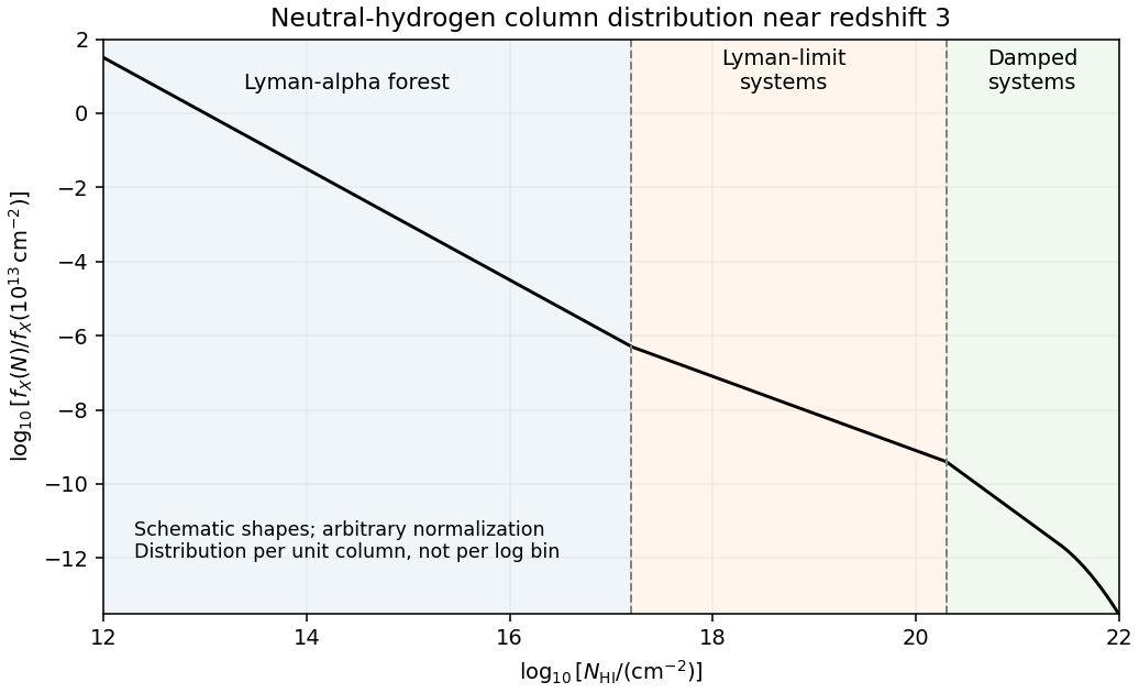
Schematic neutral-hydrogen column distribution showing the forest, optically thick Lyman-limit systems and damped systems
. Details. This sketch shows representative shapes and transition scales, not an observational fit; its ordinate is distribution per unit column, not counts per logarithmic bin. In an Einstein-de Sitter universe, , so a fixed comoving population with fixed physical cross-section above a fixed column threshold has . ThusThe observed redshift evolution of the Lyman-alpha forest is much stronger for commonly selected forest lines. For example, Kim, Cristiani and D'Odorico's absorption survey finds an index about in for over , corresponding to an increase by approximately . This number is selection-dependent. Expansion changes the gas density, and the evolving cosmic ionizing background changes its neutral fraction through photoionization equilibrium, moving systems across a fixed neutral-column threshold. Structure also evolves. A non-evolving population with fixed physical cross-section is therefore not an adequate physical model of the observed forest.
Past exam of the mathematics course of the University of Cambridge 2004 iii Paper 66 4 i Solution by Codex 0 2026-10-14
Codex 0 2026-10-14An isolating integral is a single-valued integral of motion whose fixed value confines an orbit to a lower-dimensional level set of phase space. Along the flow, ; for an autonomous Hamiltonian, this means . Several isolating integrals are independent when their gradients are linearly independent on the regular region considered. Counting them requires a specified domain: merely local orbit labels in a flow box do not establish global single-valued integrals. The following cases concern regular globally meaningful orbit constraints.
Past exam of the mathematics course of the University of Cambridge 2004 iii Paper 53 2 5 Solution by Codex 0 2026-10-14
Codex 0 2026-10-14Each independent run uses one oracle call and gives a uniformly sampled equation . Collect linearly independent equations and use Gaussian elimination over . Their solution space has dimension one and consists of , so the promised nonzero solution identifies uniquely.
To quantify the expected query count for Simon sampling, write . If the existing equations have rank , their span contains of the possible samples. A fresh equation raises the rank with probability . The mean waiting time is the corresponding geometric distribution mean, givingThe last sum is less than : its first term is and its remaining terms are bounded by . Hence the expected number of quantum queries is . For a fixed high-confidence budget, use samples. Failure to span means that a nonzero linear functional on the -dimensional sampling space annihilates every sample. Each such functional has probability , so the union bound gives failure probability at most . Thus queries suffice for failure probability at most . For , the nonzero string is known already and no samples are needed.
Classically, a collision between distinct queried arguments immediately yields . Random queries produce this collision after order calls, by the birthday problem. Conversely, choose the nonzero period uniformly and label the fibres randomly. Before a collision, queries can exclude at most periods, their pairwise argument differences; every remaining period has the same no-collision transcript distribution. When , those exclusions occupy a vanishing fraction of the candidate periods, and neither collision discovery nor guessing a remaining period has a constant success probability. More quantitatively, conditioned on no previous collision, the next query tests at most of at least remaining periods; summing these conditional probabilities proves the same square-root lower bound. Therefore the optimal bounded-error classical query count is , exponentially larger in than the quantum count.
Pinned article: Introduction to the OurBigBook Project
Welcome to the OurBigBook Project! Our goal is to create the perfect publishing platform for STEM subjects, and get university-level students to write the best free STEM tutorials ever.
Everyone is welcome to create an account and play with the site: ourbigbook.com/go/register. We belive that students themselves can write amazing tutorials, but teachers are welcome too. You can write about anything you want, it doesn't have to be STEM or even educational. Silly test content is very welcome and you won't be penalized in any way. Just keep it legal!
Intro to OurBigBook
. Source. We have two killer features:
- topics: topics group articles by different users with the same title, e.g. here is the topic for the "Fundamental Theorem of Calculus" ourbigbook.com/go/topic/fundamental-theorem-of-calculusArticles of different users are sorted by upvote within each article page. This feature is a bit like:
- a Wikipedia where each user can have their own version of each article
- a Q&A website like Stack Overflow, where multiple people can give their views on a given topic, and the best ones are sorted by upvote. Except you don't need to wait for someone to ask first, and any topic goes, no matter how narrow or broad
This feature makes it possible for readers to find better explanations of any topic created by other writers. And it allows writers to create an explanation in a place that readers might actually find it.
Figure 1. Screenshot of the "Derivative" topic page. View it live at: ourbigbook.com/go/topic/derivativeVideo 2. OurBigBook Web topics demo. Source. - local editing: you can store all your personal knowledge base content locally in a plaintext markup format that can be edited locally and published either:This way you can be sure that even if OurBigBook.com were to go down one day (which we have no plans to do as it is quite cheap to host!), your content will still be perfectly readable as a static site.
- to OurBigBook.com to get awesome multi-user features like topics and likes
- as HTML files to a static website, which you can host yourself for free on many external providers like GitHub Pages, and remain in full control

Figure 2. You can publish local OurBigBook lightweight markup files to either OurBigBook.com or as a static website.
Figure 3. Visual Studio Code extension installation.
Figure 5. . You can also edit articles on the Web editor without installing anything locally. Video 3. Edit locally and publish demo. Source. This shows editing OurBigBook Markup and publishing it using the Visual Studio Code extension. 
- Infinitely deep tables of contents:



All our software is open source and hosted at: github.com/ourbigbook/ourbigbook
Further documentation can be found at: docs.ourbigbook.com
Feel free to reach our to us for any help or suggestions: docs.ourbigbook.com/#contact